PMP 40ans : une analyse textuelle de la production

Compter les mots

Author

CB MB SB

Published

June 29, 2023

Code
#tool box
library(tidyverse) #on ne peut plus s'en passer
library(quanteda) # les bases du nlp
library(quanteda.textstats)
library(quanteda.textmodels)
library(scales)
library(ggwordcloud)
library(ggrepel) #gestion des labels
library(ggraph) 
library(ggcorrplot)
library(flextable)
library(Rtsne)
# Import des fontes du système - cela peut être long
#font_import()
#fonts() # Liste des polices disponibles
#loadfonts(device = "pdf") # Indiquer device = "pdf" pour produire un pdf 

theme_set(theme_minimal())

# en fait on fait en noir et blanc

col<- c("purple", "#ca7dcc","#fb6a4a","orange",
        "#67000d", "firebrick","coral1" ,"pink", 
        "ivory3" , "grey","brown4", "skyblue", "blue", "darkblue", 
        "black","darkgreen", "chartreuse3", "chartreuse1")

Le problème

Analyser les thématiques de recherche de la revue PMP qui fête ses 40 ans et qui se définit ainsi :

“Depuis sa fondation en 1983 par Patrick Gibert et Jean-Claude Thoenig, la revue Politiques et Management Public a pour objectif de publier des recherches rendant compte scientifiquement de tous les aspects des fonctionnements et des évolutions des organisations publiques au sens large – Etat et collectivités territoriales, administrations hospitalières, agences, entreprises publiques et concessionnaires, associations… – mais aussi du développement et des transformations de l’action publique, que celle-ci soit sectorielle ou transversale, européenne, nationale ou locale. Revue académique trimestrielle Politiques et Management Public entend favoriser la diversité et l’originalité des approches, empiriques, théoriques, nationales ou comparatives, mono ou pluridisciplinaires. Par ses publications et l’organisation de rencontres, la revue a vocation à animer les débats sur les mutations des organisations publiques, les évolutions de leur gestion et les formes traditionnelles ou renouvelées de l’action publique. Politiques et Management Public s’adresse au milieu académique mais aussi à un large public de responsables politiques, administratifs et associatifs.”

Données

Au préalable un pré-traitement sous la forme d’une correction semi-automatique des erreurs de typographie (OCR et hyphénation), de graphie (orthographe), de ponctuation (guillemets et symbole), d’accentuation. 4 heures de travail.

Code
PMP <- read_csv("data/PMPLast3.csv", 
    locale = locale(encoding = "WINDOWS-1252"))
dn<-PMP %>% 
  select(Key,`Publication Year`,Title, `Abstract Note`, Issue, Volume)%>% 
  rename(Year=`Publication Year`, Abstract=`Abstract Note`) %>% 
  mutate(text=paste0(Title,". ", Abstract),
         nchar=nchar(text),
         n_words = stringr::str_count(text, ' ')+1,
         decade=ifelse(Year<1990,"1980",
              ifelse(Year>1989 & Year<1995,"1990",
                ifelse(Year>1994 & Year<2000,"1995",
                       ifelse(Year>1999 & Year<2005,"2000",
                              ifelse(Year>2004 & Year<2010,"2005",
                                  ifelse(Year>2009 & Year<2015,"2010",
                                          ifelse(Year>2014 & Year<2020,"2015","2020"))))))), 
         Issue2=ifelse(str_sub(Issue, 1,3)=="Vol",str_sub(Issue, -1),Issue), 
         Issue2=ifelse(Issue2=="1-2",1, ifelse(Issue2=="3-4",3, Issue2)),
         x=as.numeric(Issue2)/4,
         numéro=Year+x)

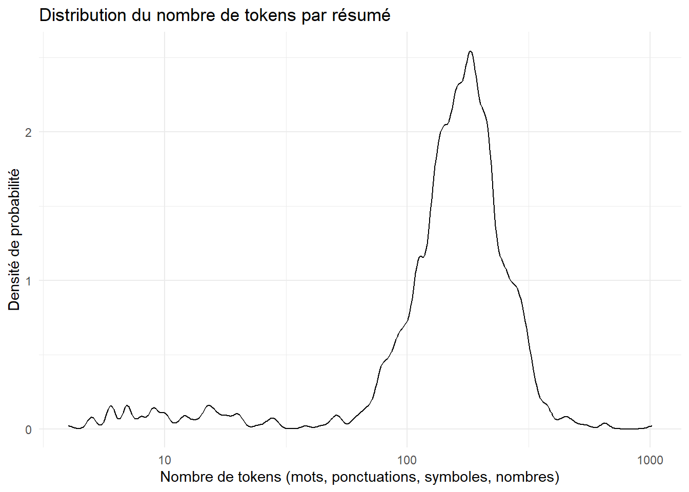
La taille des résumés

L’unité textuelle est le résumé que complète le titre en première phrase.

Code
ggplot(dn, aes(x=n_words))+
#  geom_histogram(binwidth = 10)+
  geom_density(adjust = .5)+
  theme_minimal()+
  labs(title= "Distribution du nombre de tokens par résumé", 
       x="Nombre de tokens (mots, ponctuations, symboles, nombres)",
       y="Densité de probabilité")+
  scale_x_log10()

Code
# filtrage du corpus

dn<- dn%>%filter(n_words>50 & n_words<1000)

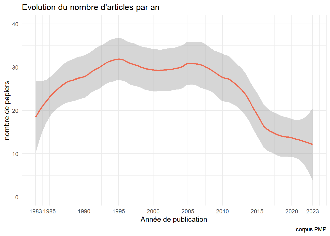
Evolution de la production

Un cycle de vie typique ? Croissance, maturité , déclin avec un tournant en 2005 ? La difficulté à alimenter la revue ?

Code
dn_year<-dn %>% 
  group_by(Year) %>% 
  summarise(n_abs=n(),n_words=sum(n_words))

ggplot(dn_year, aes(x=Year,y=n_abs))+
  geom_smooth(method = "loess",span=.35, color="Coral2")+
  labs(title="Evolution du nombre d'articles par an",
       y="nombre de papiers",
       x="Année de publication",caption="corpus PMP")+
  scale_x_continuous(breaks=c(1983, 1985,1990,1995,2000,2005,2010, 2015, 2020, 2023))+
  ylim(0,40)

Code
ggsave("./images/pmp_n_articles_an.jpeg", width = 27, height = 18, units = "cm")

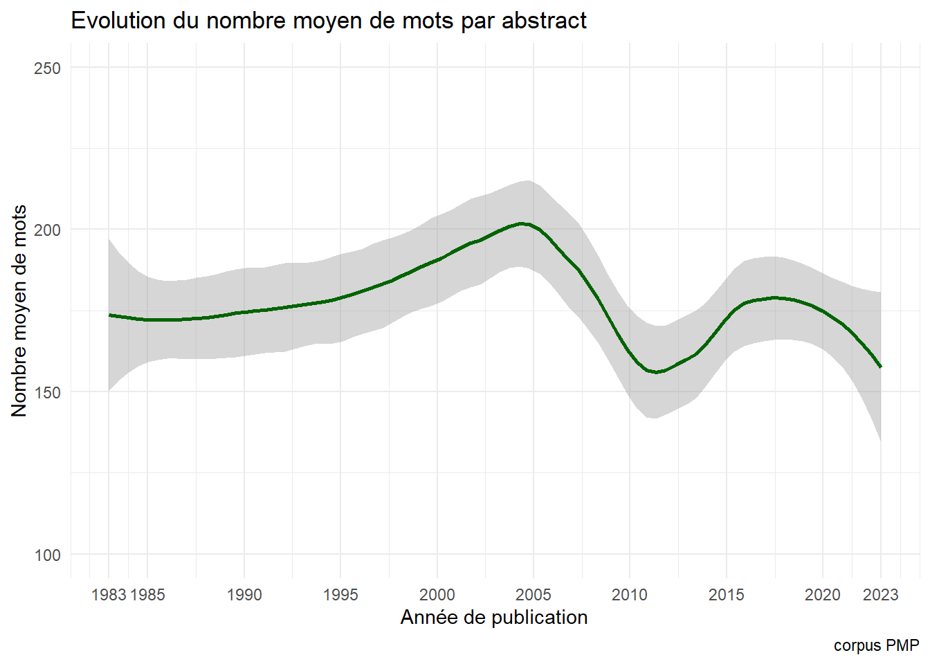
Stabilité de la taille des résumés

le manque des mots-clés

Code
ggplot(dn_year, aes(x=Year,y=n_words/n_abs))+
  geom_smooth(method = "loess",span=.4,color="darkgreen")+
  labs(title="Evolution du nombre moyen de mots par abstract",
       y="Nombre moyen de mots",
       x="Année de publication",caption="corpus PMP")+
  scale_x_continuous(breaks=c(1983, 1985,1990,1995,2000,2005,2010, 2015, 2020, 2023))+
  ylim(100,250)

Code
ggsave("./images/evol1.jpeg", width = 27, height = 18, units = "cm")

Analyse globale du lexique

On va compter les mots du corpus en otant les stopwords. On cherche à identifier les expressions par une méthode de collocation.

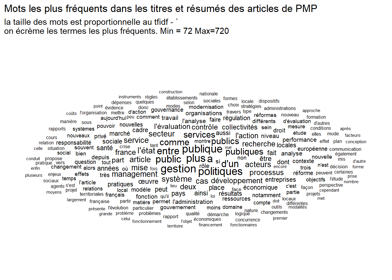
en tfidf pour pondérer la généralité. Certains mots se retrouvent dans tous les textes, s’ils sont fréquents ils sont aussi très peu distinctifs.

collocations

Avec les collocations parce que ce type de langage favorise les expressions composées : par exemple “service public”

Code
# tokenization
corp<-corpus(dn$text, docvars =dn)
toks <- tokens(corp, remove_punct = TRUE, padding=TRUE)%>% 
 tokens_select(pattern = stopwords('french'), selection = 'remove')

#collocation

tstat_col_caps <- 
  tokens_select(toks, case_insensitive = TRUE,
                                padding = TRUE) %>% 
           textstat_collocations(min_count = 7, size=2:5)%>%
  filter(lambda>8 & z>4) %>% as.data.frame()

ft<-flextable(tstat_col_caps)
ft <- theme_vanilla(ft)
ft <- add_footer_lines(ft, "")
ft <- color(ft, part = "footer", color = "#666666")
ft <- set_caption(ft, caption = "Les collocations principales")

ft
Les collocations principales

collocation

count

count_nested

length

lambda

z

point vue

45

43

2

8.536141

29.679882

certain nombre

34

34

2

8.506113

26.788840

après avoir

30

30

2

8.004512

26.553477

l'union européenne

46

46

2

8.391365

26.302951

ressources humaines

43

42

2

8.352612

24.195753

société civile

26

26

2

8.959132

22.517874

dès lors

19

9

2

8.377991

22.451935

d'enseignement supérieur

22

22

2

9.031043

22.132721

l'enseignement supérieur

19

19

2

9.215335

19.811301

lutte contre

20

20

2

9.544281

19.522958

chefs d'établissement

13

13

2

9.946444

18.079851

fonds structurels

11

11

2

9.041801

17.086587

conseils régionaux

9

8

2

8.259906

17.017276

agences régionales

8

8

2

8.258098

16.833122

pôles compétitivité

8

7

2

8.721656

16.731339

partenariats public-privé

8

8

2

8.545502

16.702842

organique relative

9

9

2

8.878311

16.627208

dernières décennies

11

10

2

8.068072

16.559098

grille lecture

8

8

2

9.156477

16.448836

000 habitants

8

8

2

9.583954

16.057066

conseils généraux

7

7

2

8.458335

16.046254

montée puissance

9

9

2

9.453216

16.031715

d'europe centrale

11

11

2

9.334018

15.878622

partant constat

7

3

2

8.259972

15.808042

remise cause

16

16

2

9.609750

15.749403

interne externe

7

7

2

8.015173

15.170090

tableau bord

8

8

2

9.671906

15.126337

compte tenu

13

13

2

8.207781

14.829054

années 80

21

21

2

8.274159

14.242873

parties prenantes

28

28

2

12.782629

13.819189

retour d'expérience

7

6

2

9.194979

13.604784

difficultés rencontrées

7

7

2

8.053824

13.221343

effets pervers

11

11

2

8.115455

13.146903

d'autre part

75

26

2

10.640097

12.839484

marges manœuvre

10

10

2

11.784248

12.314343

court terme

8

8

2

8.972732

12.247791

hauts fonctionnaires

15

15

2

10.010822

11.568065

marché intérieur

10

10

2

8.034939

11.348505

système éducatif

21

20

2

8.678206

10.251890

sous l'angle

9

9

2

9.049935

10.227464

orientée vers

8

8

2

8.949837

10.034514

tableaux bord

14

11

2

12.937328

8.748989

balanced scorecard

8

8

2

14.137954

8.472798

centrale orientale

11

11

2

11.531276

7.913503

loi organique

16

16

2

10.979263

7.621525

ad hoc

8

8

2

15.236574

7.508658

part entière

8

8

2

9.178040

6.300029

Un dictionnaire

On intègre ces expressions dans le vocabulaire. et avec quelques manipulations on établit le dictionnaire.

Code
#integration dans le lexique
toks_comp <- tokens_compound(toks, pattern = tstat_col_caps) 

#dfm
dfm <-  dfm(toks_comp)

# Dictionnaire et métriques
tstat_freq <- as.data.frame(textstat_frequency(dfm))

# La taille du lexique
N<-as.numeric(nrow(tstat_freq))
# Le nombre de token 
M=sum(tstat_freq$frequency)
# Le calcul des statistique
tstat_freq<-tstat_freq %>% 
  mutate(idf=log(N/docfreq),
         tfidf=(frequency/M)*idf)
min=72
max=720
#on sélectionne les rank premiers 
tstat_freq2<- tstat_freq %>%
  filter(frequency> min & frequency <max) #420

#une illustration 
set.seed(42)
ggplot(tstat_freq2, aes(label = feature, size = tfidf)) +
  geom_text_wordcloud() +
  scale_size_area(max_size = 5) +
  scale_color_discrete()+
  labs(title="Mots les plus fréquents dans les titres et résumés des articles de PMP",
       subtitle = paste0("la taille des mots est proportionnelle au tfidf - `\non écrème les termes les plus fréquents. Min = ", min, " Max=",max),
       caption=NULL)

Code
ggsave("./images/lexic2.jpeg", width = 27, height = 18, units = "cm")

Il comprend x termes différents.

Evolution dans le temps : un critère de keyness

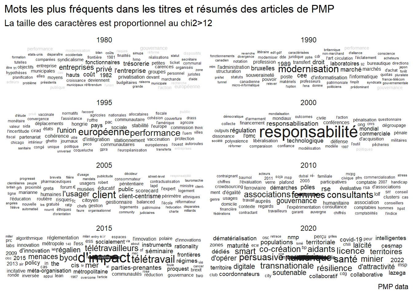
On peut donner la même représentation par groupe quinquénal, mais ce n’est pas assez discriminant. Une analyse en keyness serait sans doute meilleure

Code
quant_deca<- toks_comp %>% 
  tokens_group(groups = decade)
  
dfm<- quant_deca %>%dfm() %>% 
  dfm_group(groups=decade)

chi<-12
keyness1980<-textstat_keyness(dfm, target = "1980") %>%as.data.frame()%>% mutate(decade="1980")%>%filter(abs(chi2)>chi)
keyness1990<-textstat_keyness(dfm, target = "1990") %>%as.data.frame()%>% mutate(decade="1990")%>%filter(abs(chi2)>chi)
keyness1995<-textstat_keyness(dfm, target = "1995") %>%as.data.frame()%>% mutate(decade="1995")%>%filter(abs(chi2)>chi)
keyness2000<-textstat_keyness(dfm, target = "2000") %>%as.data.frame()%>% mutate(decade="2000")%>%filter(abs(chi2)>chi)
keyness2005<-textstat_keyness(dfm, target = "2005") %>%as.data.frame()%>% mutate(decade="2005")%>%filter(abs(chi2)>chi)
keyness2010<-textstat_keyness(dfm, target = "2010") %>%as.data.frame()%>% mutate(decade="2010")%>%filter(abs(chi2)>chi)
keyness2015<-textstat_keyness(dfm, target = "2015") %>%as.data.frame()%>% mutate(decade="2015")%>%filter(abs(chi2)>chi)
keyness2020<-textstat_keyness(dfm, target = "2020") %>%as.data.frame()%>% mutate(decade="2020")%>%filter(abs(chi2)>chi)

keyness<-rbind(keyness1980, keyness1990,keyness1995, keyness2000, keyness2005, keyness2010, keyness2015,keyness2020)

keyness$decade=as.factor(keyness$decade)

ggplot(keyness, aes(label=feature, group=decade))+
  geom_text_wordcloud(aes(label=feature,size=chi2), color=ifelse(keyness$chi2>0, "grey10", "grey80")) +
  scale_size_area(max_size = 7) +
  labs(title="Mots les plus fréquents dans les titres et résumés des articles de PMP",
       subtitle = paste0("La taille des caractères est proportionnel au chi2>", chi),
       caption="PMP data")+
  facet_wrap(~decade, ncol=2)

Code
ggsave("./images/keyness_word0.jpeg", width = 27, height = 18, units = "cm")

Comptons les mots

Plutôt que de compter globalement, on va compter analytiquement. On va chercher des catégories précises. en saisissant les mots par des regex, ou expression régulières. Ce sont de petite formule qui permettent de trouver des pattern particulier. Une date par exemple qui s’exprime dans une forme xx/xx/xxx où les x sont des chiffres. Dans notre cas prenons l’exemple du terme “organisation”. il peut prendre de nombreuses formes ( morphologie): organisation, organisations, organisationnel,organisationnelle, organisationnelles, Organisation … On va donc compter les mots avec cette méthode qui permet de saisir une grande part de la variété morphologique qu’il prennent dans le texte.

Il faut aussi se doter d’une métrique. Certains sont peu fréquents, d’autres le sont plus, mais cela dépend aussi du volume : un mot peut être plus fréquent simplement par ce qu’il y a plus de mots prononcés dans le segment d’étude, il faut donc normaliser en rapportant la fréquence des mots dans le segment t, au nombres de mots produit au temps t. C’est une mesure de densité.On la calcule au niveau du texte, on la moyenne à l’année, et on la lisse par une méthode de loess avec un span de 0.45.

Une petite ontologie

Avant de compter il faut construire des catégories. On les retrouvera techniquement par des méthode de regex pour saisir la variété des morphèmes et des flexions.

Ce qui caractérise la revue s’est une dualité politiques publique et management public, le premier terme se construisant dans l’idée que l’état agit sur la société et l’économie par des politiques publiques, qui souvent sont sectorielles, et dont les contenus et orientation doté d’une sorte de permanence (par la norme et le droit), sont redéfini par la force politique. Le second se rapporte au fait organisationnel, celui qui se manifeste dans le corps de l’état, ses administrations, ses agences dont la finalité est justement la mise en oeuvre des premières.

Politiques publiques -> Institution->Management Public -> Performance et organisations

flowchart LR

Institutions[Institutions] --> Management[Management]

PP[Politiques Publiques] --> Management[Management]

Institutions[Institutions] --> PP[Politiques Publiques]

PP[Politiques Publiques] --> Performance[Performance]

Management[Management]--> Performance[Performance]

Epoque[Epoque] --> Management[Management]

Epoque[Epoque] --> Institutions[Institutions]

Chacune de ces catégories se déclinent en concepts, puis en termes, et sont opérationalisés par des regex qui permettent d’en capturer les variations.

flowchart TD

Catégories[Catégories] --> Concept[Concepts]

subgraph 2

Catégories[Catégories] --> éléments1[Eléments du \nmanagement]

Catégories[Catégories] --> éléments2[Institutions]

Catégories[Catégories] --> éléments3[Performances]

Catégories[Catégories] --> éléments4[Politiques Publiques]

end

subgraph 1

Concept[Concept] --> Termes1[Termes]

end

Termes1[Termes] --> subs[Substantifs …]

subgraph 0

Termes1[Termes] --> Regex[Regex]

subs[Substantifs …]--> Regex[Regex]

end

autre tentative

Code
#pour les lissages

span<-0.45

Les catégories que l’on va suivre sont les suivantes

Politiques et Management publics?

Les éléments du management public

Code
#champs
dn$PolitiquePublique<-str_count(dn$text, pattern = "[P|p]olitique.*\\s[P|p]ublique.*")/dn$n_words
dn$Administration<-str_count(dn$text, pattern = "[A|a]dmini.*")/dn$n_words
dn$Gestion<-str_count(dn$text, pattern = "[G|g]estion.*")/dn$n_words
dn$Management<-str_count(dn$text, pattern = "[M|m]anag.*")/dn$n_words
dn$ServicePublic<-str_count(dn$text, pattern = "[S|s]ervice.*[:blank:][P|p]ubli.*")/dn$n_words
dn$Juridique<-str_count(dn$text, pattern = "[J|j]u[r|d|s][i|t].*")/dn$n_words+
  str_count(dn$text, pattern = "[D|r]roit.*")/dn$n_words
#fonctions
dn$Marketing<-str_count(dn$text, pattern = "[M|m]arket.*")/dn$n_words+
  str_count(dn$text, pattern = "[M|m]arque.*")/dn$n_words
dn$RH<-str_count(dn$text, pattern = "[RH|rh].*")/dn$n_words+
  str_count(dn$text, pattern = "[R|r]essources.*.*[:blank:][H|u]main.*")/dn$n_words
dn$Stratégie<-str_count(dn$text, pattern = "[S|s]trat.*")/dn$n_words
dn$Comptabilité<-str_count(dn$text, pattern = "[C|c]ompta.*")/dn$n_words
dn$Projet<-str_count(dn$text, pattern = "[P|r]ojet.*")/dn$n_words
dn$Finance<-str_count(dn$text, pattern = "[F|f]inanc.*")/dn$n_words
dn$Numérique<-str_count(dn$text, pattern = "[N|u]méri.*")/dn$n_words+
  str_count(dn$text, pattern = "[I|i]nformati[q,c]m[u,i].*")/dn$n_words+
  str_count(dn$text, pattern = "[I|i]nformatisat.*")/dn$n_words

foo<-dn %>% 
  group_by(Year)%>% 
  summarise(Administration= mean(Administration),
            Juridique= mean(Juridique, na.rm=TRUE),
            PolitiquePublique=mean(PolitiquePublique, na.rm=TRUE),
            Gestion=mean(Gestion, na.rm=TRUE),
            Management=mean(Management, na.rm=TRUE),
            ServicePublic=mean(ServicePublic, na.rm=TRUE),
            Marketing=mean(Marketing, na.rm=TRUE),
            RH=mean(RH, na.rm=TRUE),
            Stratégie=mean(Stratégie, na.rm=TRUE),
            Comptabilité=mean(Comptabilité, na.rm=TRUE),
            Projet=mean(Projet, na.rm=TRUE),
            Finance=mean(Finance, na.rm=TRUE),
            Numérique=mean(Numérique, na.rm=TRUE),
            ) 

foo1<-foo%>%
  pivot_longer(-Year, names_to = "keyword",values_to = "n")

foo2<-foo1 %>%
  group_by(keyword)%>%
  summarise(Densité=mean(n, na.rm=TRUE),
#            min=quantile(n, probs= 0.25),
#            max=quantile(n, probs= 0.75),
             m=n(),
             se=sd(n)/sqrt(m))

ggplot(foo2, aes(x=reorder(keyword, Densité), y=Densité))+
  geom_bar(stat="identity", fill="Grey65")+
  geom_errorbar(aes(ymin=Densité-se, ymax=Densité+se), width=.2,
                 position=position_dodge(.9)) +
    scale_y_continuous(labels=scales::percent,limits=c(0, NA))+
  coord_flip()+ 
  labs(title="Fréquence de citations des termes clés", 
              subtitle="Les éléments du management public",
       x=NULL)

Code
ggsave("./images/keyword11.jpeg", width = 27, height = 18, units = "cm")
Code
foo3<-foo %>%
  select(2:14)

r<-cor(foo3)

ggcorrplot(r, hc.order = TRUE, type = "lower",
   outline.col = "white",
   colors = c("Grey80", "white","Grey80" ) , lab=TRUE, lab_size=2, tl.cex=9)+
  labs(title="Matrice des corrélations temporelles des termes clés",
       subtitle = "Les éléments du management public")

Code
ggsave("./images/keyword12.jpeg", width = 27, height = 18, units = "cm")
Code
foo1<-foo1 %>%left_join(foo2)
ggplot(foo1, aes(x=Year, y=n, group=keyword))+
  geom_smooth(method="loess", alpha=0, span=span, aes(color=keyword), linewidth=0.5)+
  scale_colour_grey()+
  scale_y_continuous(labels=scales::percent,limits=c(0, NA))+
  labs(y="densité", 
       x=NULL, 
       title = "Fréquence des termes",
       subtitle="Les éléments du management public")+
  facet_wrap(vars(keyword), scale="free")+
  theme(legend.position="none")+theme(axis.text.y = element_text(size = 7,angle = 0),
                                      axis.text.x = element_text(size = 7,angle = 0))

Code
ggsave("./images/keyword13.jpeg", width = 27, height = 18, units = "cm")

tsne

Code
d<- 1-r

#library(Rtsne)
tsne_out <- Rtsne(d, perplexity=3) # Run TSNE
set.seed(123)
TSNE<-cbind(tsne_out$Y,rownames(d)) %>%as.data.frame() %>%
  rename(keyword=3)%>%
  left_join(foo2)
TSNE$V1<-as.numeric(TSNE$V1)
TSNE$V2<-as.numeric(TSNE$V2)
ggplot(TSNE,aes(x=V1, y=V2,label=V3))+
  geom_text_repel(aes(label=keyword,size=log10(Densité)))+
  theme(legend.position="none")+
  labs(title="Fréquence de citation des termes clés",
       subtitle=" Les éléments du management public",
       x=NULL, y=NULL,
       caption = "Modèle Tsne - perplexité=5\nsur D=1-r")

Code
ggsave("./images/keyword14.jpeg", width = 27, height = 18, units = "cm")

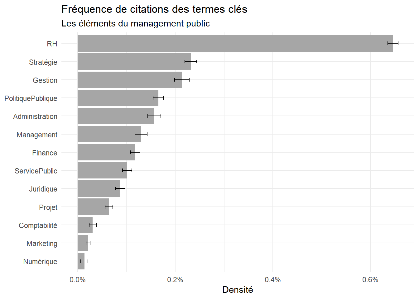
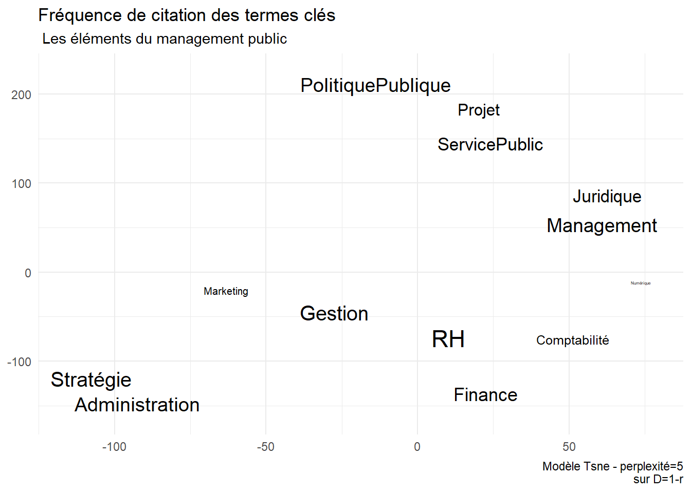
les Ressources Humaines dominent, sa densité est de 0.8% quand pour les autres elle est de 0.2%. le management public est d’abord considéré dans cette ressources par la lentille de la ressource humaine. Le corps de l’état est une chair de fonctionnaires. C’est une obsession constante.

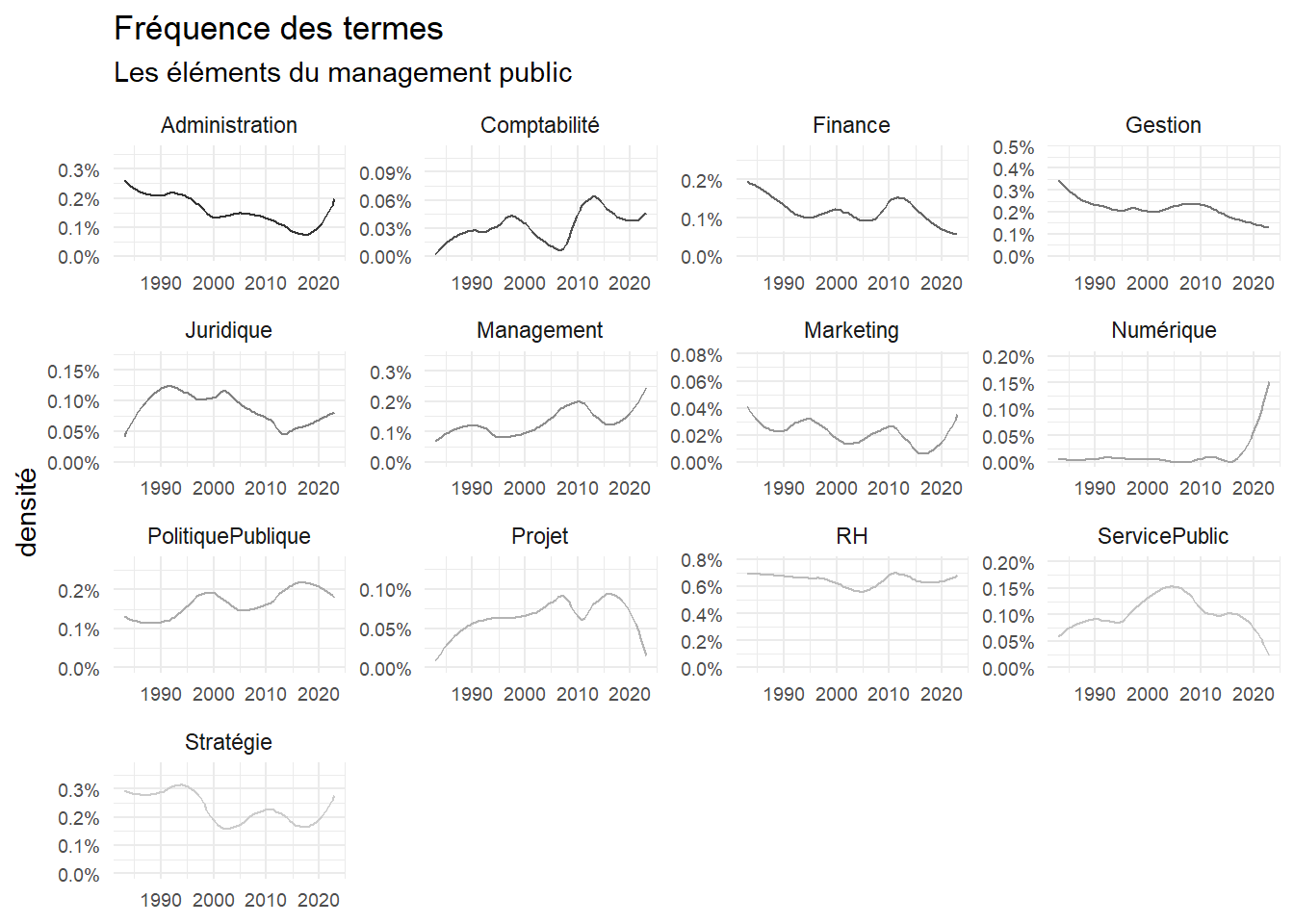
le management et la stratégie gagnent du terrain.

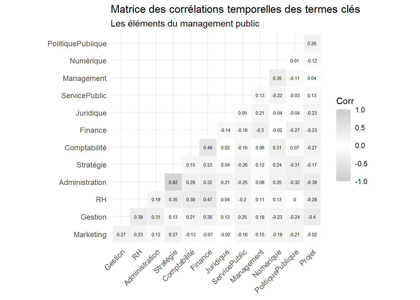
le management croît, l’administration décline , peut-être un sursaut, la stratégie et le management progresse, la gestion recule ? les politiques publique prennent un peu d’importance.

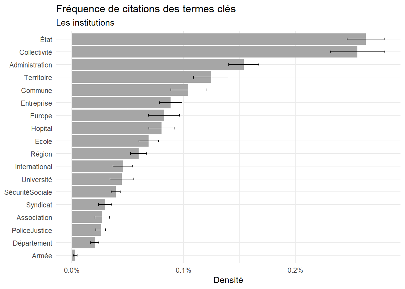
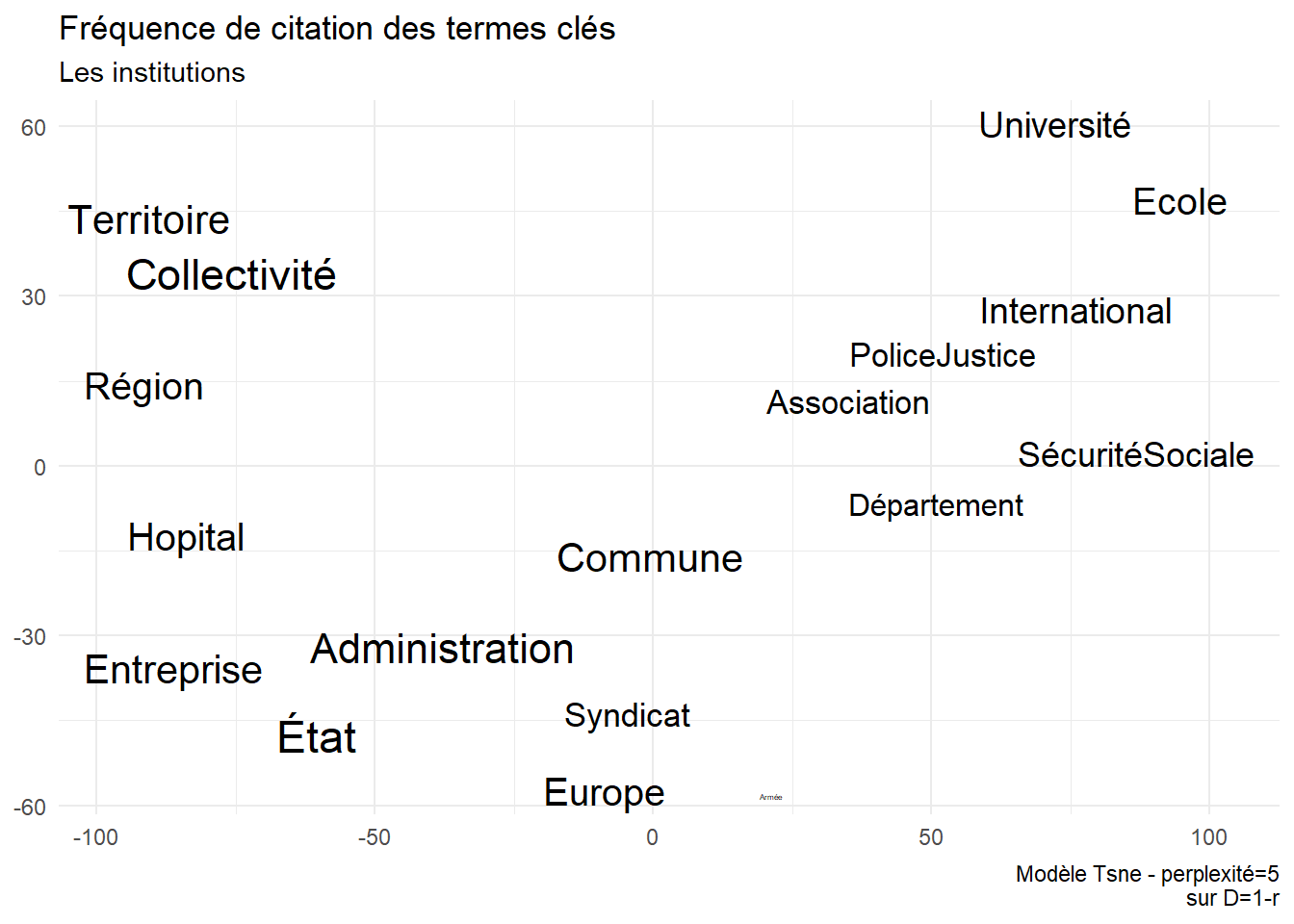
Institutions et champs

  • Institutions internationales
  • Etat
  • région
  • Collectivité locales et communales, local,métropole, mairie, municipalité
  • PPP
  • Agence
  • services publics
Code
#Nation
dn$Etat<-str_count(dn$text, pattern = "[E|é|É]tat.*")/dn$n_words+
  str_count(dn$text, pattern = "[G|g]ouverne.*")/dn$n_words
dn$Administration<-str_count(dn$text,"[A|a]dministrat.*")/dn$n_words+
  str_count(dn$text,"[P|r]éfe[c|r].*")/dn$n_words

#Local
dn$Collectivité<-str_count(dn$text, pattern = "[C|c]ollectivit.*")/dn$n_words+
  str_count(dn$text,".*[L|l]oca.*")/dn$n_words
dn$Région<-str_count(dn$text, pattern = "[R|r][é|e]gion.*")/dn$n_words
dn$Département<-str_count(dn$text, pattern = "[D|d][é|e]partement.*")/dn$n_words
dn$Territoire<-str_count(dn$text,"[T|t][e|é]rrit[o, oi].*")/dn$n_words
dn$Commune<-str_count(dn$text,".*[C|c]ommun[e,al].*")/dn$n_words+
  str_count(dn$text, pattern = "[M|m]unicip.*")/dn$n_words
dn$Entreprise<-str_count(dn$text,".*[E|n]trepr[e|is].*")/dn$n_words+
  str_count(dn$text, pattern = "[P|p]priv.*")/dn$n_words
dn$Association<-str_count(dn$text,".*[A|a]ssocia.*")/dn$n_words+
  str_count(dn$text, pattern = "ONG.*")/dn$n_words
dn$Syndicat<-str_count(dn$text,".*[S|s]yndica.*")/dn$n_words +
  str_count(dn$text, pattern = "[F|f]édéra.*")/dn$n_words
dn$Université<-str_count(dn$text,"[U|u]niversit.*")/dn$n_words
dn$Ecole<-str_count(dn$text,"[E|é|É]col.*")/dn$n_words+ 
  str_count(dn$text,"[E|e|É]nseign.*")/dn$n_words
dn$Hopital<-str_count(dn$text, pattern = "[H|h][ô|o][.|s]pital.*")/dn$n_words+
  str_count(dn$text, pattern = "[S|a]nté.*")/dn$n_words
dn$PoliceJustice<-str_count(dn$text,"[P|p]olic.*")/dn$n_words+ 
  str_count(dn$text,"[J|u]stic.*")/dn$n_words
dn$Armée<-str_count(dn$text,"[A|a]rmé.*")/dn$n_words+
  str_count(dn$text,"[M|m]ilitai.*")/dn$n_words
dn$SécuritéSociale<-str_count(dn$text,"[S|s]écur.*[S|s]ocia.*")/dn$n_words+
  str_count(dn$text,"[U|r][S|s][A|a].*")/dn$n_words+
  str_count(dn$text,"[A|a][N|n][E|e].*")/dn$n_words
           
#international
dn$Europe<-str_count(dn$text, pattern = "[E|e]urop.*")/dn$n_words
dn$International<-str_count(dn$text,"[I|i]nterna.*")/dn$n_words

foo<-dn %>% 
  group_by(Year)%>% 
  summarise(Collectivité=mean(Collectivité, na.rm=TRUE),
            Région=mean(Région, na.rm=TRUE),
            Département=mean(Département, na.rm=TRUE),
            État=mean(Etat, na.rm=TRUE),
            Europe=mean(Europe, na.rm=TRUE),
            International=mean(International, na.rm=TRUE),
            Territoire=mean(Territoire, na.rm=TRUE),
            Administration=mean(Administration, na.rm=TRUE),
            Commune=mean(Commune, na.rm=TRUE),
            Entreprise=mean(Entreprise, na.rm=TRUE),
            Association=mean(Association, na.rm=TRUE),
            Syndicat=mean(Syndicat, na.rm=TRUE),
            Université =mean(Université, na.rm=TRUE),
            Hopital =mean(Hopital, na.rm=TRUE),
            Ecole =mean(Ecole, na.rm=TRUE),
            PoliceJustice=mean(PoliceJustice, na.rm=TRUE),
            Armée=mean(Armée, na.rm=TRUE),
            SécuritéSociale= mean(SécuritéSociale, na.rm=TRUE)
  )


foo1<-foo%>%
  pivot_longer(-Year, names_to = "keyword",values_to = "n")

foo2<-foo1 %>%
  group_by(keyword)%>%
  summarise(Densité=mean(n, na.rm=TRUE),
#            min=quantile(n, probs= 0.25),
#            max=quantile(n, probs= 0.75),
             m=n(),
             se=sd(n)/sqrt(m))

ggplot(foo2, aes(x=reorder(keyword, Densité), y=Densité))+
  geom_bar(stat="identity", fill="Grey65")+
  geom_errorbar(aes(ymin=Densité-se, ymax=Densité+se), width=.2,
                 position=position_dodge(.9)) +
    scale_y_continuous(labels=scales::percent,limits=c(0, NA))+
  coord_flip()+ 
  labs(title="Fréquence de citations des termes clés", 
              subtitle="Les institutions",
       x=NULL)

Code
ggsave("./images/keyword21.jpeg", width = 27, height = 18, units = "cm")

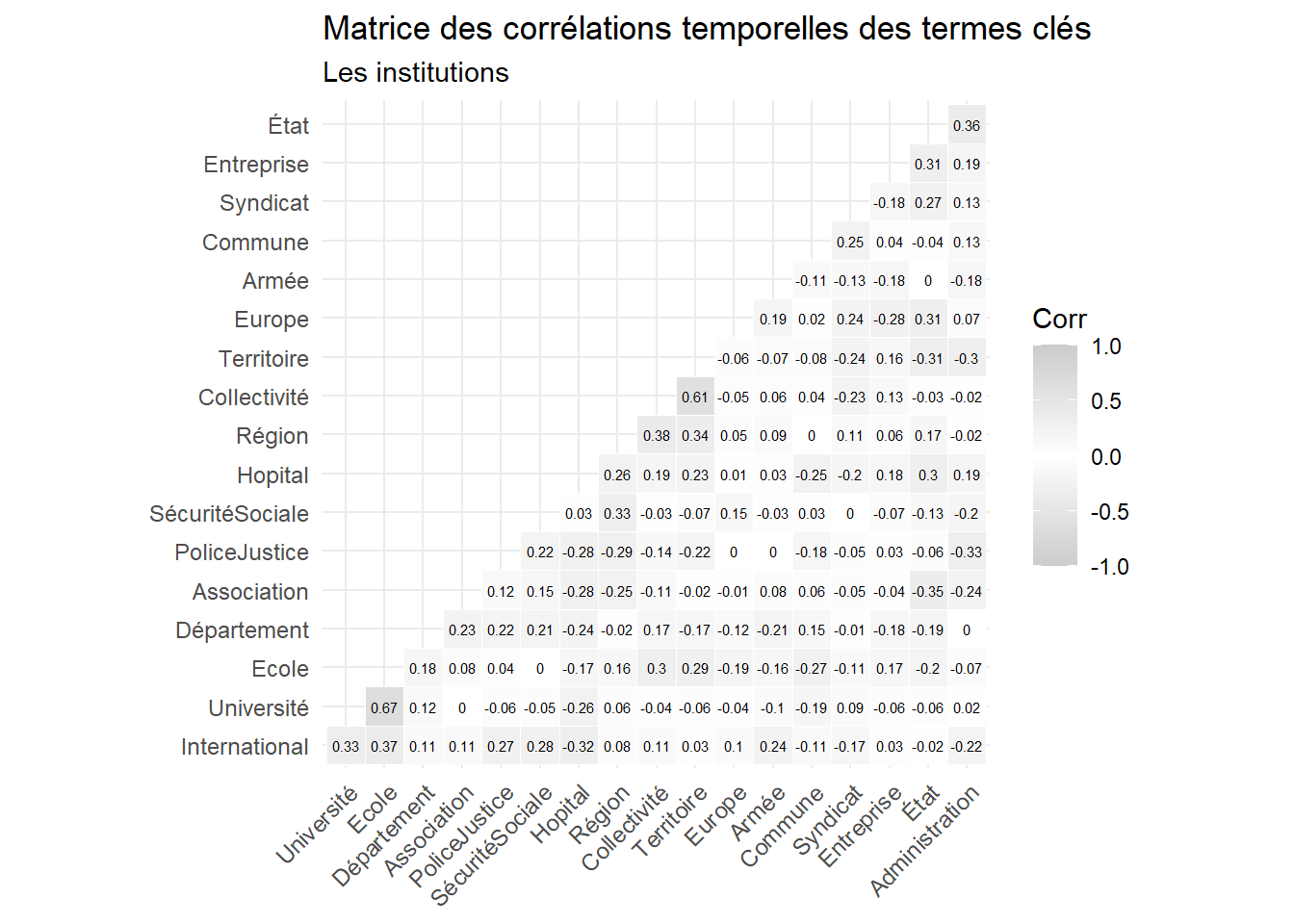
Corrélations des citations d’institutions

Code
foo3<-foo %>%
  select(2:19)

r<-cor(foo3)

ggcorrplot(r, hc.order = TRUE, type = "lower",
   outline.col = "white",
   colors = c("Grey80", "white","Grey80" ) , lab=TRUE, lab_size=2, tl.cex=9)+
  labs(title="Matrice des corrélations temporelles des termes clés",
       subtitle = "Les institutions")

Code
ggsave("./images/keyword22.jpeg", width = 27, height = 18, units = "cm")

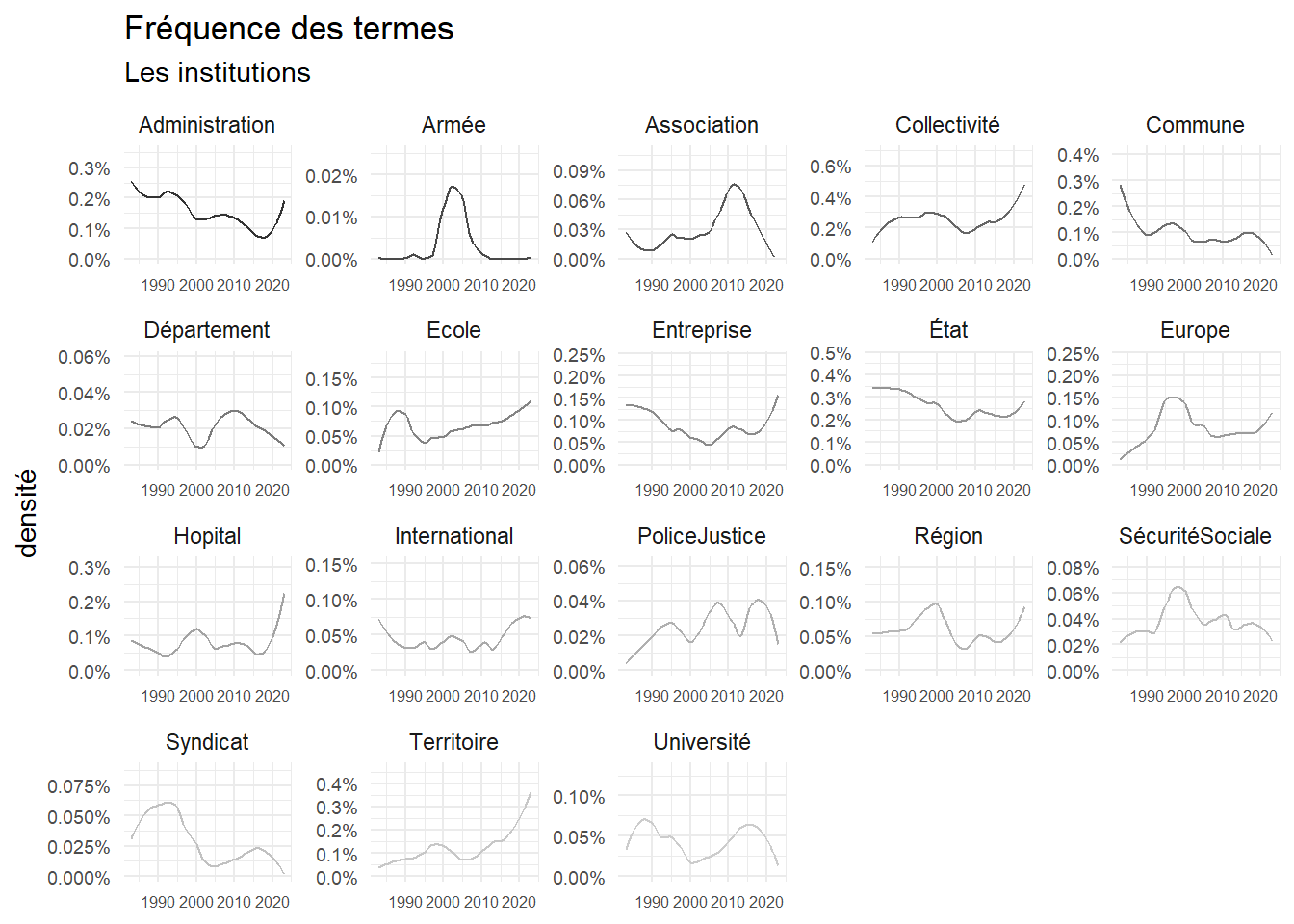
Evolution

Code
foo1<-foo1 %>%left_join(foo2)
ggplot(foo1, aes(x=Year, y=n, group=keyword))+
  geom_smooth(method="loess", alpha=0, span=span, aes(color=keyword), linewidth=.5)+
  scale_colour_grey()+
  scale_y_continuous(labels=scales::percent,limits=c(0, NA))+
  labs(y="densité", 
       x=NULL, 
       title = "Fréquence des termes",
       subtitle = "Les institutions")+facet_wrap(vars(keyword), scale="free")+
  theme(legend.position="none")+theme(axis.text.y = element_text(size = 7,angle = 0),
                                      axis.text.x = element_text(size = 6,angle = 0))

Code
ggsave("./images/keyword23.jpeg", width = 27, height = 18, units = "cm")

tsne

Code
d=1-r
library(Rtsne)
tsne_out <- Rtsne(d, perplexity=5) # Run TSNE
set.seed(123)
TSNE<-cbind(tsne_out$Y,rownames(d)) %>%as.data.frame() %>%rename(keyword=3)%>%left_join(foo2)
TSNE$V1<-as.numeric(TSNE$V1)
TSNE$V2<-as.numeric(TSNE$V2)
ggplot(TSNE,aes(x=V1, y=V2,label=V3))+
  geom_text_repel(aes(label=keyword,size=log10(Densité)))+
  theme(legend.position="none")+
  labs(title="Fréquence de citation des termes clés",
       subtitle="Les institutions",
       x=NULL, y=NULL,
       caption = "Modèle Tsne - perplexité=5\nsur D=1-r")

Code
ggsave("./images/keyword24.jpeg", width = 27, height = 18, units = "cm")

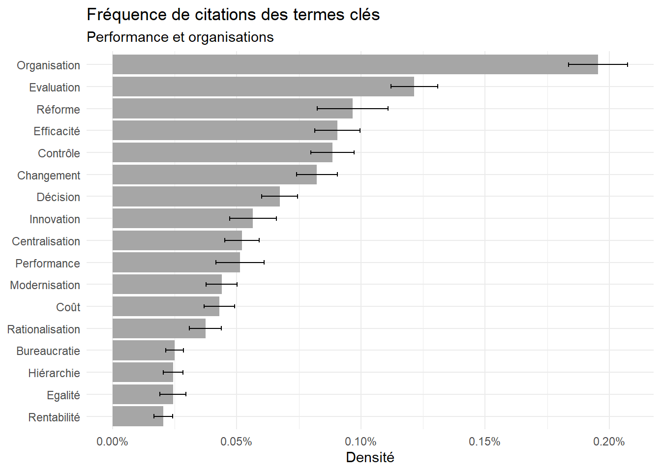
la performance et l’organisation

Les problèmes :

  • modernisation et réforme, changement, planification

  • efficacité/ performance /contrôle / rationalisation/ outcome efficience effectivité: RENDEMENT, coûts, rentabilité évaluation, mesure, indicateur, contrôle, équité, égalité, analyse de politique

  • Organisation, Administration, hiérarchie, bureaucratie, Décentralisation/ décentralisation

  • communs, participation

  • financement, finance

  • opération, exécution, décision, projet

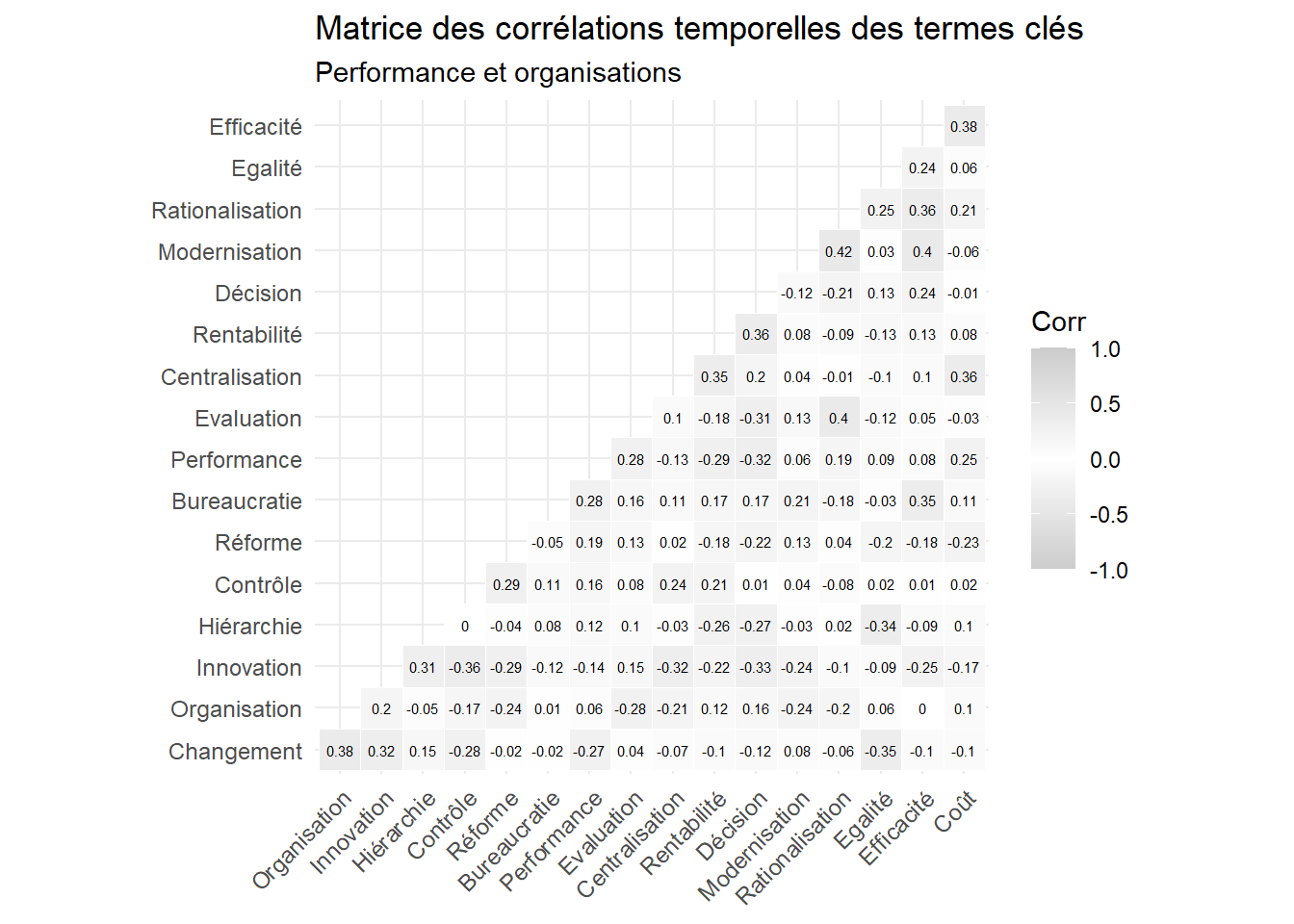
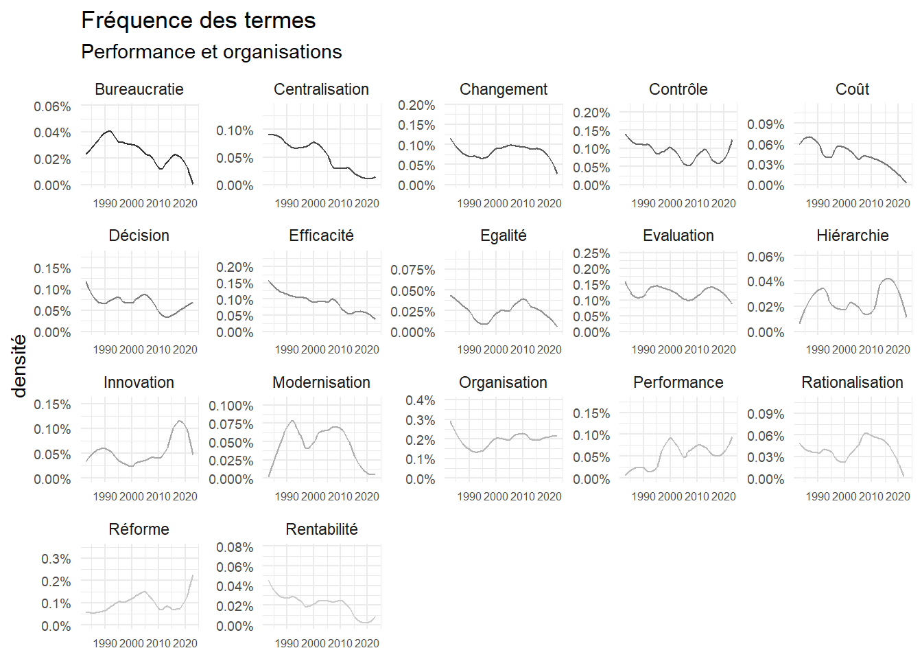
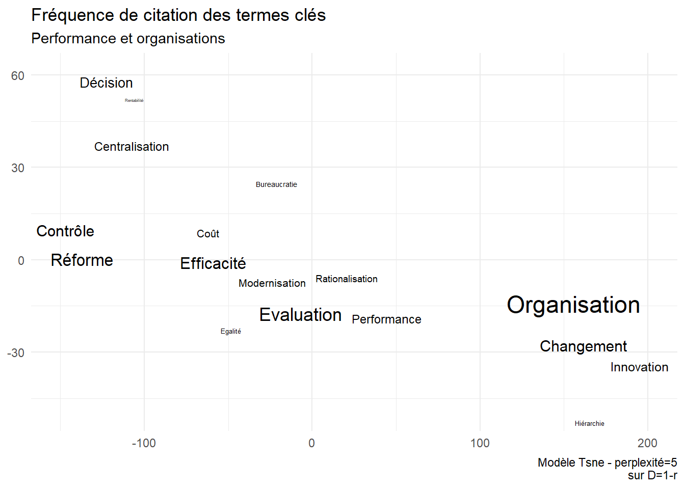
Les éléments “Performance et organisation”

Code
#performance

dn$Performance<-str_count(dn$text,"[P|p]erform.*")/dn$n_words
dn$Rentabilité<-str_count(dn$text,"[R|r]entab.*")/dn$n_words
dn$Efficacité<-str_count(dn$text,"[E|e|É]fficac.*")/dn$n_words+
  str_count(dn$text,"[E|e|É]fficien.*")/dn$n_words
dn$Rentabilité<-str_count(dn$text,"[R|r]entab.*")/dn$n_words+
  str_count(dn$text,"[P|p]rofit.*")/dn$n_words+
  str_count(dn$text,"[R|r]endemen.*")/dn$n_words
dn$Coûts<-str_count(dn$text,"[C|c]oût.*")/dn$n_words
dn$Egalité<-str_count(dn$text,"[E|é|É]quit.*")/dn$n_words+
  str_count(dn$text,"[E|é|É]galit.*")/dn$n_words

dn$Evaluation<-str_count(dn$text,"[E|é|É]valu.*")/dn$n_words
dn$Controle<-str_count(dn$text,"[C|c]ontrôl.*")/dn$n_words

dn$Réforme<-str_count(dn$text,"[R|r]éform.*")/dn$n_words
dn$Modernisation<-str_count(dn$text,"[M|m]odern.*")/dn$n_words
dn$Rationalisation<-str_count(dn$text,"[R|r]ationali.*")/dn$n_words

dn$Innovation<-str_count(dn$text,"[I|i]nnov.*")/dn$n_words
dn$Organisation<-str_count(dn$text,"[O|o]rganis.*")/dn$n_words
dn$Bureaucratie<-str_count(dn$text,"[B|b]ureau.*")/dn$n_words
dn$Hiérarchie<-str_count(dn$text,"[H|h]i[é|e]rarc.*")/dn$n_words
dn$Décision<-str_count(dn$text,"[D|d]écision.*")/dn$n_words
dn$Centralisation<-str_count(dn$text,"[C|c]entrali.*")/dn$n_words
dn$Changement<-str_count(dn$text,"[C|c]hangem.*")/dn$n_words


foo<-dn %>% 
  group_by(Year)%>% 
  summarise(Performance=mean(Performance, na.rm=TRUE),
            Rentabilité=mean(Rentabilité, na.rm=TRUE),
            Efficacité=mean(Efficacité, na.rm=TRUE),
            Evaluation=mean(Evaluation, na.rm=TRUE),
            Coût=mean(Coûts, na.rm=TRUE),
            Egalité=mean(Egalité, na.rm=TRUE),
            Contrôle=mean(Controle, na.rm=TRUE),
            Réforme=mean(Réforme, na.rm=TRUE),
            Modernisation=mean(Modernisation, na.rm=TRUE),
            Rationalisation=mean(Rationalisation, na.rm=TRUE),
            Innovation=mean(Innovation, na.rm=TRUE),
            Changement=mean(Changement, na.rm=TRUE),
            Organisation=mean(Organisation, na.rm=TRUE),
            Hiérarchie=mean(Hiérarchie, na.rm=TRUE),
            Bureaucratie=mean(Bureaucratie, na.rm=TRUE),
            Décision=mean(Décision, na.rm=TRUE),
            Centralisation=mean(Centralisation, na.rm=TRUE)
            ) 

foo1<-foo%>%
  pivot_longer(-Year, names_to = "keyword",values_to = "n")

foo2<-foo1 %>%
  group_by(keyword)%>%
  summarise(Densité=mean(n, na.rm=TRUE),
#            min=quantile(n, probs= 0.25),
#            max=quantile(n, probs= 0.75),
             m=n(),
             se=sd(n)/sqrt(m))

ggplot(foo2, aes(x=reorder(keyword, Densité), y=Densité))+
  geom_bar(stat="identity", fill="Grey65")+
  geom_errorbar(aes(ymin=Densité-se, ymax=Densité+se), width=.2,
                 position=position_dodge(.9)) +
    scale_y_continuous(labels=scales::percent,limits=c(0, NA))+
  coord_flip()+ 
  labs(title="Fréquence de citations des termes clés", 
              subtitle="Performance et organisations",
       x=NULL)

Code
ggsave("./images/keyword31.jpeg", width = 27, height = 18, units = "cm")

corrélation ” Performance et organisation”

Code
foo3<-foo %>%
  select(2:18)

r<-cor(foo3)

ggcorrplot(r, hc.order = TRUE, type = "lower",
   outline.col = "white",
   colors = c("Grey80", "white","Grey80" ) , lab=TRUE, lab_size=2, tl.cex=9)+
  labs(title="Matrice des corrélations temporelles des termes clés",
       subtitle = "Performance et organisations")

Code
ggsave("./images/keyword32.jpeg", width = 27, height = 18, units = "cm")

Evolution ” Performance et organisation”

Code
foo1<-foo1 %>%left_join(foo2)
ggplot(foo1, aes(x=Year, y=n, group=keyword))+
  geom_smooth(method="loess", alpha=0, span=span, aes(color=keyword), linewidth=.5)+
  scale_colour_grey()+
  scale_y_continuous(labels=scales::percent,limits=c(0, NA))+
  labs(y="densité", 
       x=NULL, 
       title = "Fréquence des termes",
       subtitle = "Performance et organisations")+facet_wrap(vars(keyword), scale="free")+
  theme(legend.position="none")+
  theme(axis.text.y = element_text(size = 7,angle = 0),
                                      axis.text.x = element_text(size = 6,angle = 0))

Code
ggsave("./images/keyword33.jpeg", width = 27, height = 18, units = "cm")

tsne ” Performance et organisation”

Code
d<- 1-r

library(Rtsne)
tsne_out <- Rtsne(d, perplexity=2) # Run TSNE
set.seed(123)
TSNE<-cbind(tsne_out$Y,rownames(d)) %>%as.data.frame() %>%rename(keyword=3)%>%left_join(foo2)
TSNE$V1<-as.numeric(TSNE$V1)
TSNE$V2<-as.numeric(TSNE$V2)
ggplot(TSNE,aes(x=V1, y=V2,label=V3))+
  geom_text_repel(aes(label=keyword,size=Densité))+
  theme(legend.position="none")+
  labs(title="Fréquence de citation des termes clés",
       subtitle="Performance et organisations",
       x=NULL, y=NULL,
       caption = "Modèle Tsne - perplexité=5\nsur D=1-r")

Code
ggsave("./images/keyword34.jpeg", width = 27, height = 18, units = "cm")

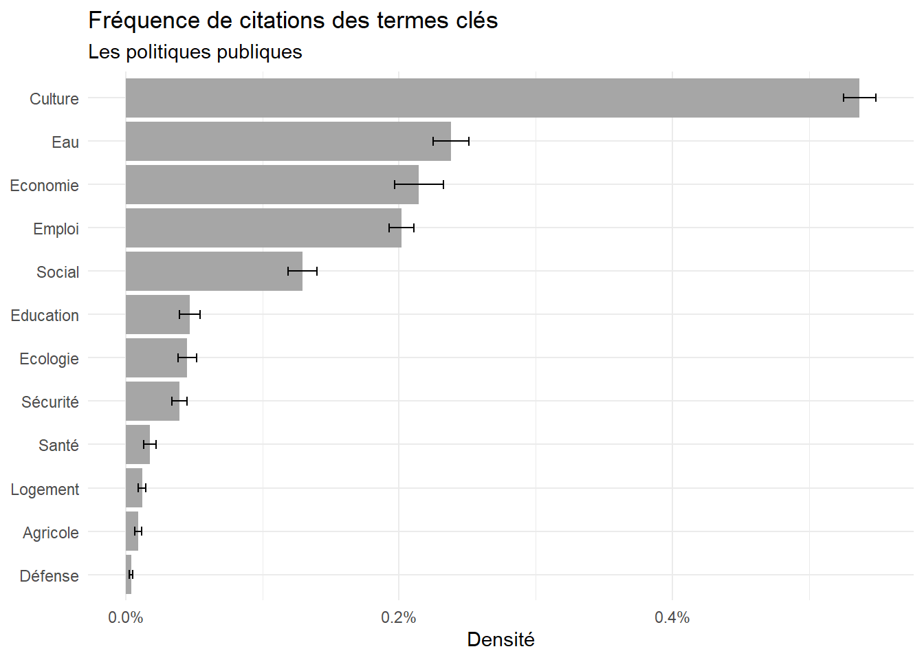
Politiques publiques

Les politiques publiques sont des combinaisons de régulations, de taxes, de discours et de subventions qui visent dans un domaine donné à un certain résultats. Les buts les moyens et les priorités peuvent être discutées, mais souvent les politiques publiques sont constantes car le problème qu’elle traite ne dépendant toujours d’une évaluation politiques, il peut être un lieu commun, par exemple la réduction des morts et des blessés de la circulation. Depuis les années 60 ce coût a été réduit par 5, par une accumulation de progrès techninque (les voiture, la conduite), et de normes souvent contraignantes concernant la consommation d’alcool, les limites de vitesses, des dispositifs de ralentissement etc.

Les politiques publiques ont leurs ve qui n’est pas forcément celle de la vie politique.

Les politiques publiques sont souvent sectorielles.

  • Recherche
  • Protection sociale
  • Retraites
  • Développement économique
  • fiscalité, dette
  • Université et enseignement étudiants université
Code
#écologie/environnement
dn$Ecologie<-str_count(dn$text,".*[É|E|e]colo.*")/dn$n_words+
  str_count(dn$text,".*[E|e]nvironnem.*")/dn$n_words+
  str_count(dn$text,".*[C|c]hasse.*")/dn$n_words

#Eau et déchets

dn$EauDéchet<-str_count(dn$text,".*[E|e]au.*")/dn$n_words+
  str_count(dn$text, pattern = "[D|d]échet.*")/dn$n_words+
  str_count(dn$text, pattern = "[O|r]dure.*")/dn$n_words+
    str_count(dn$text, pattern = "[R|r]écupéra.*")/dn$n_words

dn$Santé<-str_count(dn$text, pattern = "[S|s]an[i]t.*")/dn$n_words+
  str_count(dn$text, pattern = "[P|r]éventi.*")/dn$n_words

dn$Défense<- str_count(dn$text,".*[D|d]éfense.*")/dn$n_words +
  str_count(dn$text, pattern = "[S|s]ouverain.*\\s[N|a]tion.*")/dn$n_words

dn$Education<-str_count(dn$text,"[E|e|é|É]duc.*")/dn$n_words+
  str_count(dn$text,"[E|e]nseignementduc.*")/dn$n_words+
    str_count(dn$text,"[C|c]ollège.*")/dn$n_words

dn$Social<- str_count(dn$text,".*[S|s]ocia.*")/dn$n_words
dn$Emploi<- str_count(dn$text,".*[E|e]mp.*")/dn$n_words+ 
  str_count(dn$text,".*[C|c]h[o|ô]m.*")/dn$n_words

dn$Economie<- str_count(dn$text,".*[E|é|É|e]conomi.*")/dn$n_words+
  str_count(dn$text,".*[C|c]roissance.*")/dn$n_words+
  str_count(dn$text,".*[I|i]ndustri.*")/dn$n_words

dn$Sécurité<- str_count(dn$text,".*[S|s|É]écurité.*")/dn$n_words+
  str_count(dn$text,".*[I|i]ntérieur.*")/dn$n_words+ 
  str_count(dn$text,".*[D|d]élinqu[a|e]n.*")/dn$n_words+
  str_count(dn$text,".*[C|c]rimin.*")/dn$n_words+
  str_count(dn$text,".*[P|p]olic.*")/dn$n_words

dn$Logement<- str_count(dn$text,".*[L|l]ogemen.*")/dn$n_words+
  str_count(dn$text,".*[H|hl]abita.*")/dn$n_words

dn$Culture<- str_count(dn$text,".*[C|c]ulture.*")/dn$n_words+
  str_count(dn$text,".*[A|a]rt.*")/dn$n_words+
  str_count(dn$text,".*[M|m]usé.*")/dn$n_words+
    str_count(dn$text,".*[M|m]usi[q,c].*")/dn$n_words


dn$Agricole<- str_count(dn$text,".*[A|a]gric[u,o]l.*")/dn$n_words


foo<-dn %>% 
  group_by(Year)%>% 
  summarise(Ecologie=mean(Ecologie, na.rm=TRUE),
            Eau=mean(EauDéchet, na.rm=TRUE),
            Santé=mean(Santé, na.rm=TRUE),
            Défense=mean(Défense, na.rm=TRUE),
            Education=mean(Education, na.rm=TRUE),
            Social=mean(Social, na.rm=TRUE),
            Emploi=mean(Emploi, na.rm=TRUE),
            Economie=mean(Economie, na.rm=TRUE),
            Sécurité=mean(Sécurité, na.rm=TRUE),
            Logement=mean(Logement, na.rm=TRUE),
            Culture=mean(Culture, na.rm=TRUE),
            Agricole=mean(Agricole)
            ) 

foo1<-foo%>%
  pivot_longer(-Year, names_to = "keyword",values_to = "n")

foo2<-foo1 %>%
  group_by(keyword)%>%
  summarise(Densité=mean(n, na.rm=TRUE),
#            min=quantile(n, probs= 0.25),
#            max=quantile(n, probs= 0.75),
             m=n(),
             se=sd(n)/sqrt(m-1))

ggplot(foo2, aes(x=reorder(keyword, Densité), y=Densité))+
  geom_bar(stat="identity", fill="Grey65")+
  geom_errorbar(aes(ymin=Densité-se, ymax=Densité+se), width=.2,
                 position=position_dodge(.9)) +
    scale_y_continuous(labels=scales::percent,limits=c(0, NA))+
  coord_flip()+ 
  labs(title="Fréquence de citations des termes clés", 
              subtitle="Les politiques publiques",
       x=NULL)

Code
ggsave("./images/keyword41.jpeg", width = 27, height = 18, units = "cm")

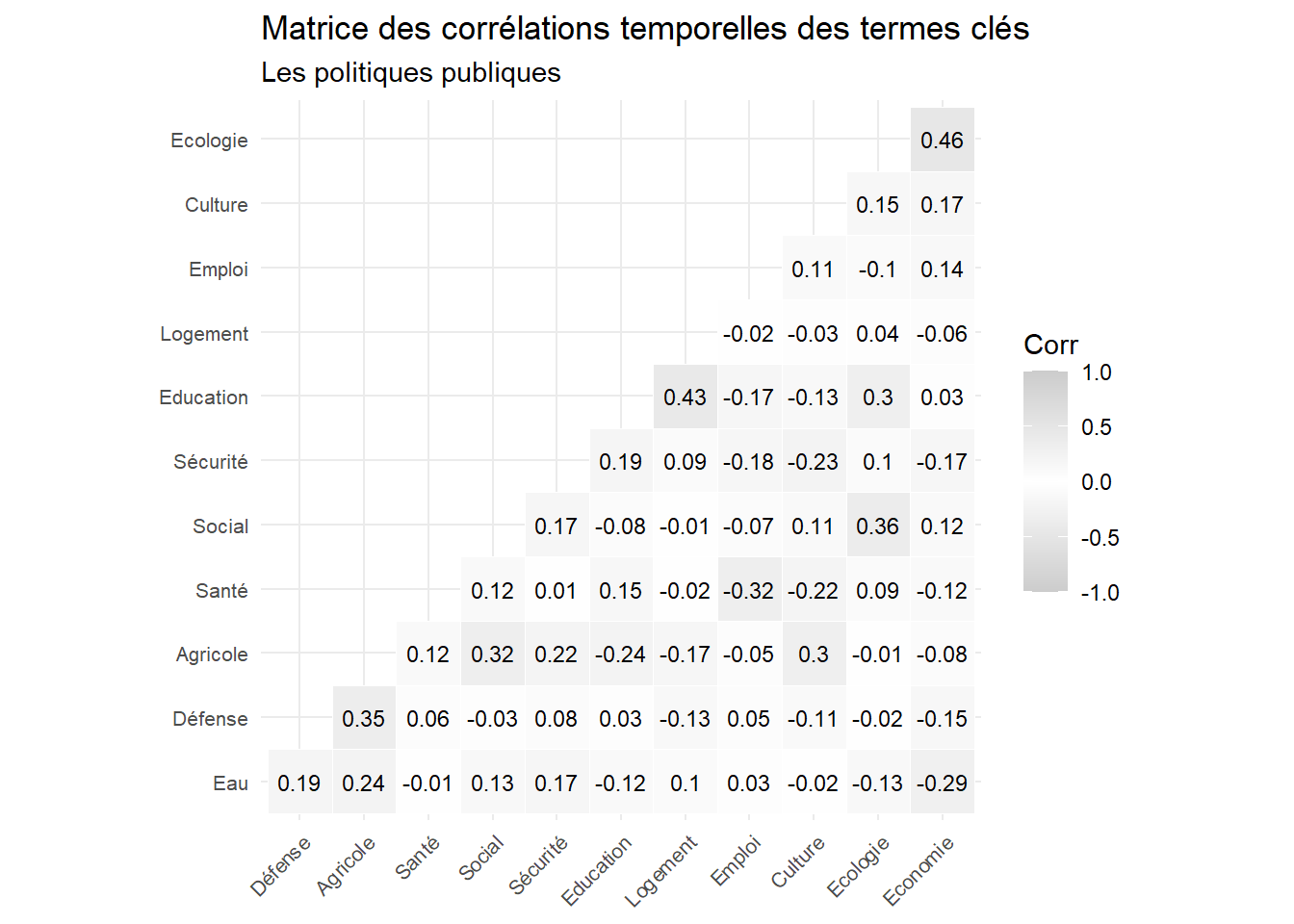
Corrélations “Politiques publiques”

Code
foo3<-foo %>%
  select(2:13) #%>% select(-6)

r<-cor(foo3)

ggcorrplot(r, hc.order = TRUE, type = "lower",
   outline.col = "white",
   colors = c("Grey80", "white","Grey80" ) , lab=TRUE, lab_size=3, tl.cex=8)+
  labs(title="Matrice des corrélations temporelles des termes clés",
       subtitle = "Les politiques publiques")

Code
ggsave("./images/keyword42.jpeg", width = 27, height = 18, units = "cm")

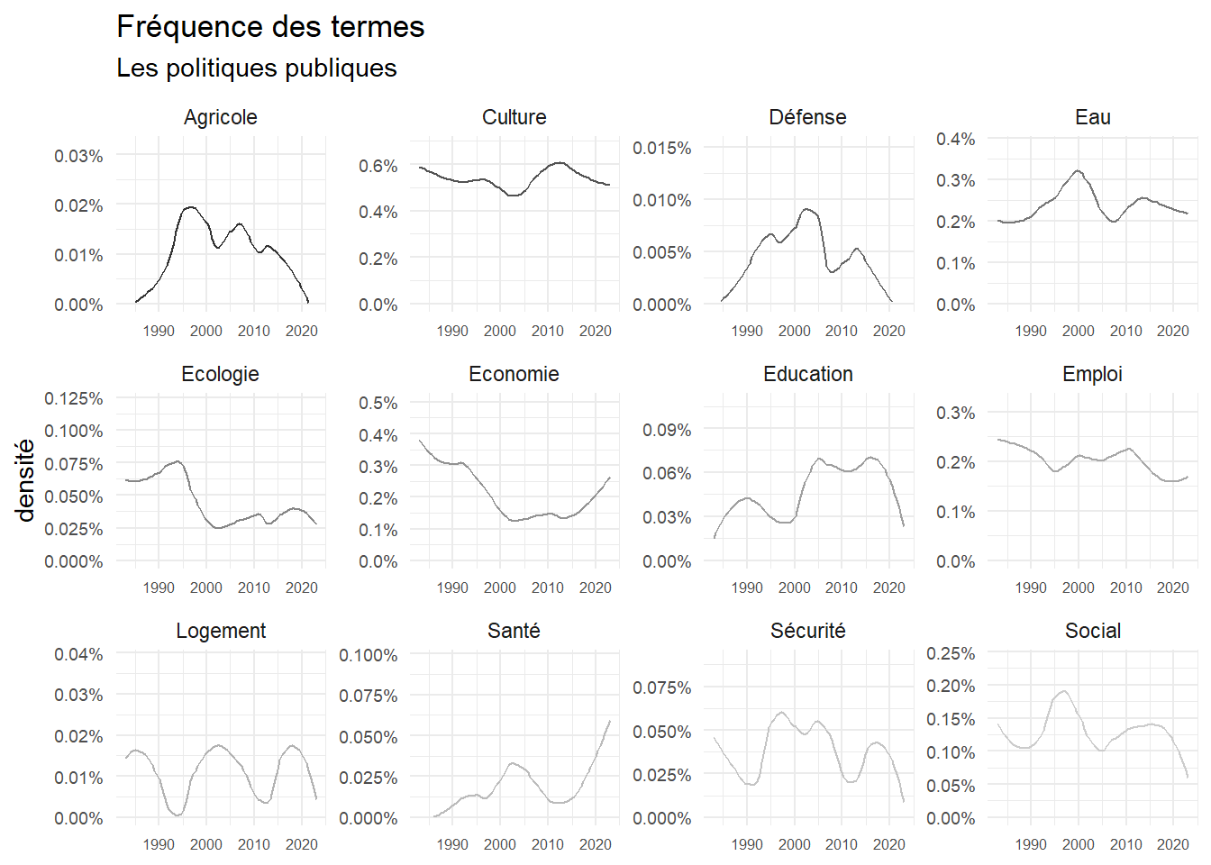
Evolution des citations ” politiques publiques”

Code
foo1<-foo1 %>%left_join(foo2)#%>%filter(keyword!="Souveraineté")

ggplot(foo1, aes(x=Year, y=n, group=keyword))+
  geom_smooth(method="loess", alpha=0, span=span, aes(color=keyword), linewidth=.5)+
  scale_colour_grey()+
  scale_y_continuous(labels=scales::percent,limits=c(0, NA))+
  labs(y="densité", 
       x=NULL, 
       title = "Fréquence des termes",
       subtitle = "Les politiques publiques")+facet_wrap(vars(keyword), scale="free")+
  theme(legend.position="none")+
  theme(axis.text.y = element_text(size = 7,angle = 0),
                                      axis.text.x = element_text(size = 6,angle = 0))

Code
ggsave("./images/keyword43.jpeg", width = 27, height = 18, units = "cm")

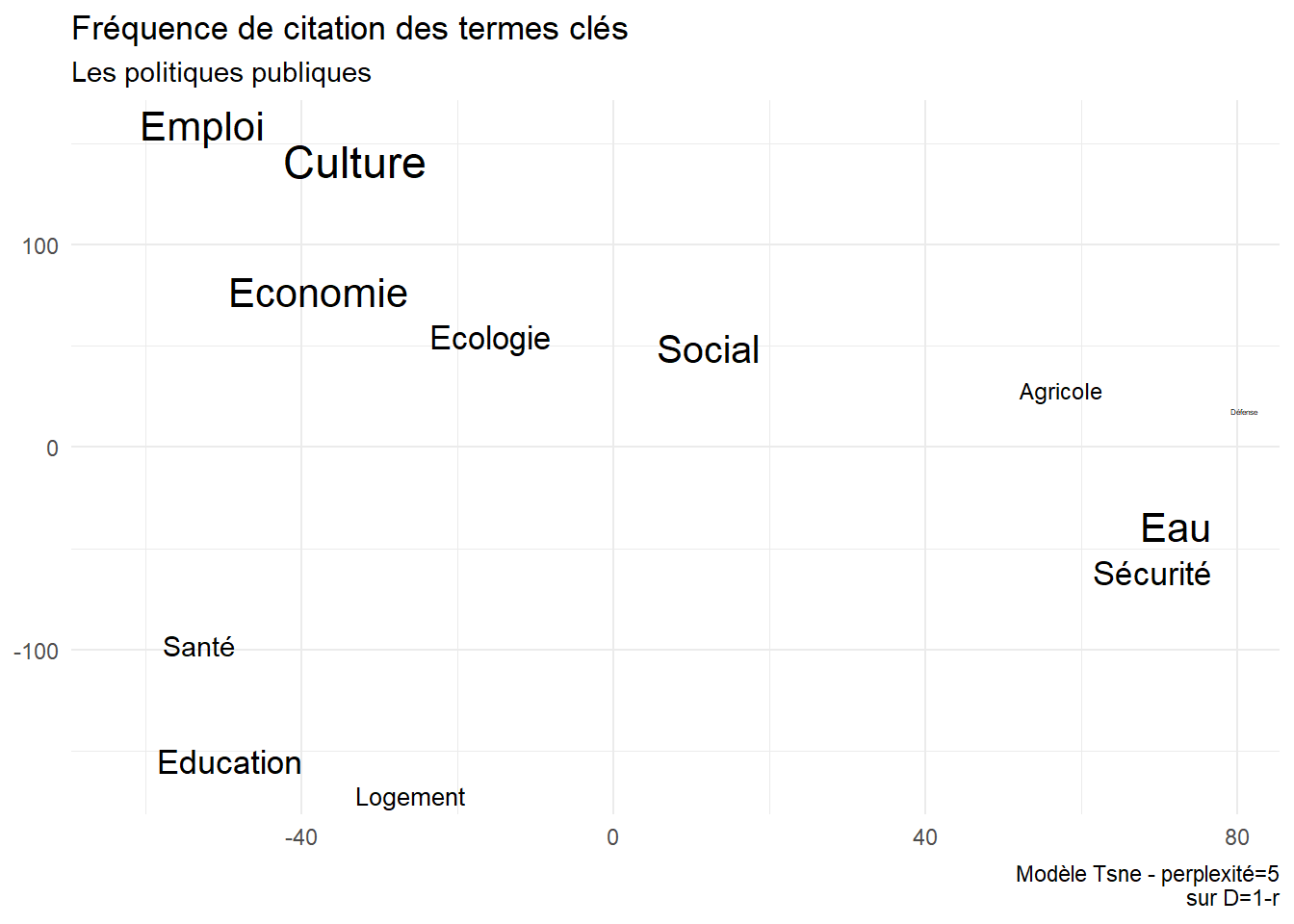
mapping des catégories “Politiques publiques”

Code
perplexité=5
d<- 1-r

library(Rtsne)
tsne_out <- Rtsne(d, perplexity=2) # Run TSNE
set.seed(123)
TSNE<-cbind(tsne_out$Y,rownames(d)) %>%as.data.frame() %>%
  rename(keyword=3)%>%
  left_join(foo2)
TSNE$V1<-as.numeric(TSNE$V1)
TSNE$V2<-as.numeric(TSNE$V2)

ggplot(TSNE,aes(x=V1, y=V2,label=V3))+
  geom_text_repel(aes(label=keyword,size=log(Densité)))+
  theme(legend.position="none")+
  labs(title="Fréquence de citation des termes clés",
       subtitle="Les politiques publiques",
       x=NULL, y=NULL,
       caption = "Modèle Tsne - perplexité=5\nsur D=1-r")

Code
ggsave("./images/keyword44.jpeg", width = 27, height = 18, units = "cm")

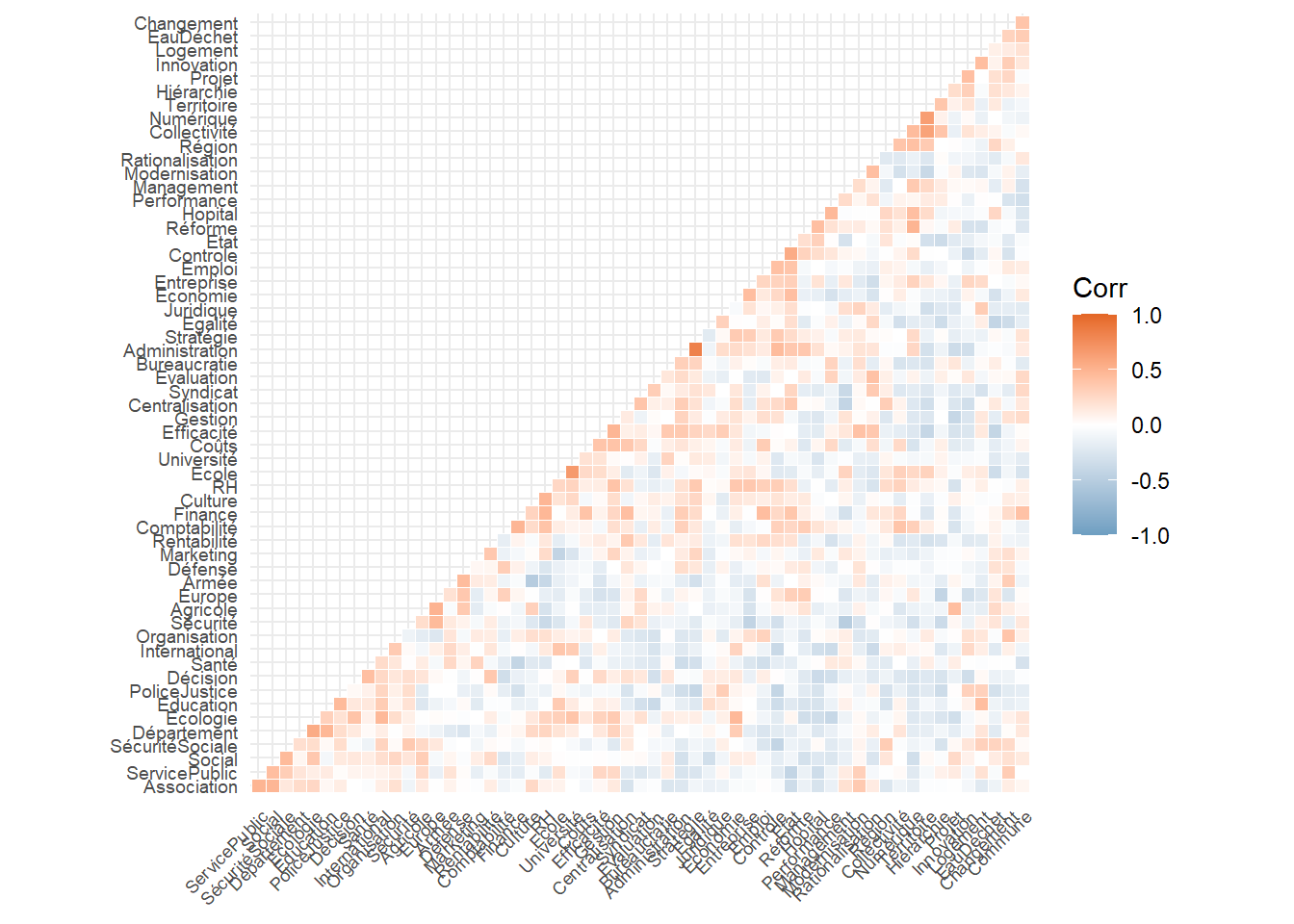
corrélations entre l’ensemble keywords

Code
foo<-dn %>%
  select(Key,Year,15:72
         ) %>% 
  pivot_longer(-c(Key, Year), names_to = "variable", values_to = "taux") %>%
  group_by(Year, variable)%>%
  summarise(taux=mean(taux, na.rm=TRUE)) %>%
  pivot_wider(Year, names_from = "variable", values_from = "taux") %>% 
  dplyr::select(-Year)
Code
r <-cor(foo[,2:59]) 

library(ggcorrplot)

ggcorrplot(r, hc.order = TRUE, type = "lower",
   outline.col = "white",
   colors = c("#6D9EC1", "white", "#E46726"), lab=FALSE, lab_size=2, tl.cex=7)

Code
ggsave("./images/keyword_cor.jpeg", width = 27, height = 18, units = "cm")

library("FactoMineR")
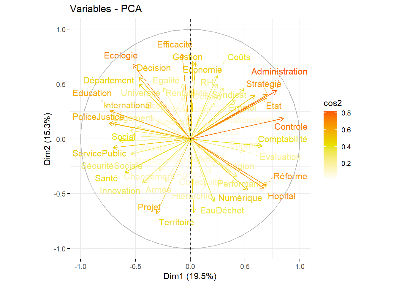
res.pca <- PCA(r, ncp=10,graph = FALSE)

library("factoextra")
eig.val <- get_eigenvalue(res.pca)

fviz_pca_var(res.pca, col.var = "cos2",
             gradient.cols = c("white", "#E7E200", "#FA5A07"),
             repel = TRUE # Évite le chevauchement de texte
             )

Code
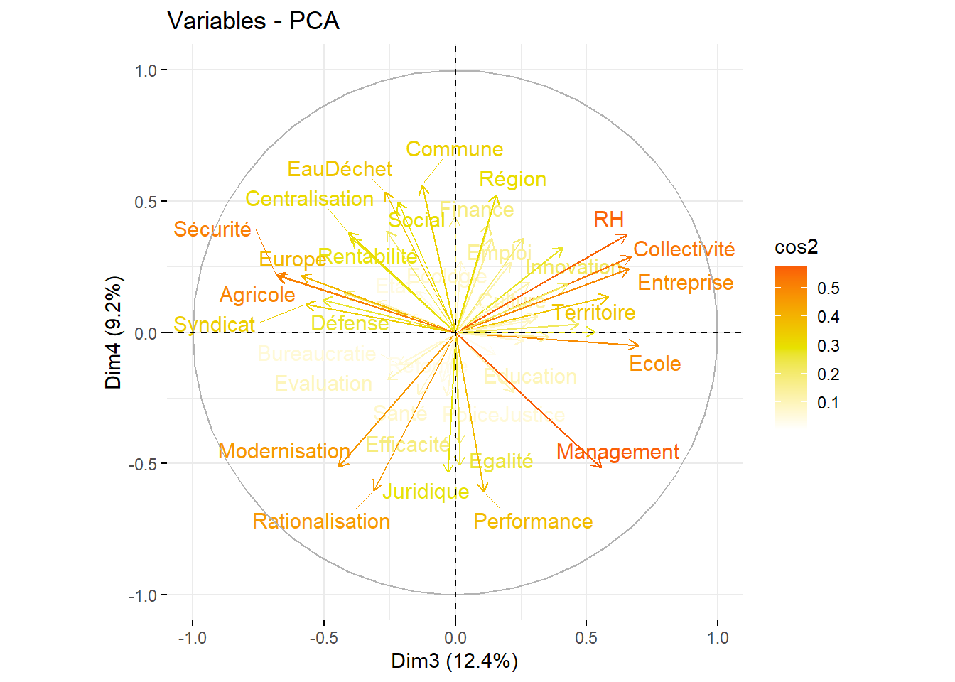
fviz_pca_var(res.pca, axes= c(3,4),col.var = "cos2",
             gradient.cols = c("white", "#E7E200", "#FA5E07"),
             repel = TRUE # Évite le chevauchement de texte
             )

Code
library(psych)

mle <- fa(r,10,rotate="oblimin",fm="uls")
summary(mle)

Factor analysis with Call: fa(r = r, nfactors = 10, rotate = "oblimin", fm = "uls")

Test of the hypothesis that 10 factors are sufficient.
The degrees of freedom for the model is 1118  and the objective function was  418.38 

The root mean square of the residuals (RMSA) is  0.07 
The df corrected root mean square of the residuals is  0.08 

 With factor correlations of 
       ULS3  ULS1  ULS5  ULS2  ULS4  ULS8  ULS6 ULS10  ULS7  ULS9
ULS3   1.00 -0.06 -0.04 -0.04 -0.09 -0.09  0.07  0.01  0.01  0.09
ULS1  -0.06  1.00 -0.11  0.03  0.01 -0.07 -0.01  0.25  0.03  0.05
ULS5  -0.04 -0.11  1.00  0.05  0.04  0.04  0.02 -0.04 -0.05  0.00
ULS2  -0.04  0.03  0.05  1.00 -0.02  0.16  0.05  0.04 -0.10 -0.01
ULS4  -0.09  0.01  0.04 -0.02  1.00  0.03  0.00  0.06  0.09 -0.04
ULS8  -0.09 -0.07  0.04  0.16  0.03  1.00  0.02 -0.02 -0.08 -0.03
ULS6   0.07 -0.01  0.02  0.05  0.00  0.02  1.00  0.06  0.00  0.03
ULS10  0.01  0.25 -0.04  0.04  0.06 -0.02  0.06  1.00 -0.04  0.05
ULS7   0.01  0.03 -0.05 -0.10  0.09 -0.08  0.00 -0.04  1.00 -0.03
ULS9   0.09  0.05  0.00 -0.01 -0.04 -0.03  0.03  0.05 -0.03  1.00
Code
fa.sort(mle,polar=FALSE)
Factor Analysis using method =  uls
Call: fa(r = r, nfactors = 10, rotate = "oblimin", fm = "uls")
Standardized loadings (pattern matrix) based upon correlation matrix
                 ULS3  ULS1  ULS5  ULS2  ULS4  ULS8  ULS6 ULS10  ULS7  ULS9
Collectivité     0.81  0.00  0.06  0.12  0.08  0.06  0.01  0.19 -0.13 -0.10
Territoire       0.68 -0.25 -0.03  0.15 -0.10 -0.23  0.11 -0.17 -0.07  0.03
Numérique        0.66  0.18 -0.18  0.01 -0.30 -0.07  0.13 -0.11  0.24  0.11
Comptabilité     0.47  0.21 -0.02  0.02 -0.12  0.14 -0.20  0.36  0.33  0.04
Région           0.42  0.07  0.09  0.08  0.25 -0.18  0.16  0.00  0.15  0.05
Hopital          0.34  0.11 -0.30 -0.33 -0.06 -0.15  0.08 -0.03  0.03 -0.09
Administration   0.04  0.85 -0.10 -0.09 -0.02 -0.01 -0.03  0.09  0.06  0.04
Stratégie        0.02  0.76  0.04  0.01 -0.01 -0.16  0.17 -0.03 -0.01  0.21
Efficacité      -0.32  0.48 -0.02  0.32 -0.08  0.10 -0.24  0.01 -0.33 -0.10
Projet          -0.13 -0.35  0.21 -0.12 -0.08 -0.32  0.04 -0.25  0.04  0.19
Modernisation   -0.32  0.35  0.20 -0.10 -0.32 -0.06 -0.33 -0.12  0.05 -0.17
Organisation    -0.06 -0.35  0.19  0.08 -0.14  0.00  0.33  0.29 -0.22 -0.10
Controle        -0.08  0.32 -0.27 -0.13 -0.18 -0.32  0.22  0.32  0.18  0.00
Changement       0.03 -0.08  0.67 -0.27 -0.11 -0.05  0.02  0.21 -0.12  0.00
Social          -0.19 -0.08  0.57  0.12  0.12 -0.06  0.26 -0.13  0.03  0.03
Egalité         -0.34 -0.22 -0.55  0.14 -0.04  0.18 -0.07  0.13 -0.05  0.09
ServicePublic   -0.13 -0.12  0.54  0.17 -0.26  0.02 -0.15 -0.02 -0.03 -0.15
Association     -0.26 -0.16  0.48  0.18 -0.36  0.03 -0.12  0.17  0.15  0.05
SécuritéSociale  0.08  0.01  0.41 -0.06  0.22  0.35  0.07 -0.21  0.20  0.11
Etat            -0.15  0.24 -0.40 -0.14  0.14  0.01  0.35  0.30  0.32  0.06
Commune         -0.02  0.05  0.37 -0.26  0.35  0.06 -0.05  0.28 -0.17  0.31
Performance      0.10 -0.03 -0.36 -0.04 -0.16 -0.27 -0.31 -0.08 -0.14 -0.05
Ecole            0.29 -0.07 -0.03  0.80 -0.17  0.03  0.06  0.00 -0.06  0.08
Université       0.01 -0.01 -0.05  0.71  0.09 -0.10  0.05  0.02  0.01  0.06
Ecologie        -0.09  0.28  0.34  0.46  0.19  0.37  0.16  0.02  0.02 -0.05
EauDéchet        0.22  0.03  0.35 -0.41  0.25 -0.20  0.12 -0.07  0.05  0.00
Marketing       -0.13  0.28  0.20 -0.38 -0.08 -0.05  0.25 -0.04 -0.28 -0.24
Décision        -0.35  0.05  0.01  0.37  0.22  0.01  0.25 -0.11  0.01 -0.31
Management       0.09  0.13  0.05  0.05 -0.75  0.04 -0.04 -0.10 -0.10 -0.07
Sécurité        -0.04 -0.18  0.01 -0.09  0.61  0.24 -0.13 -0.14  0.22 -0.17
Centralisation   0.05  0.37  0.01 -0.04  0.60 -0.08 -0.01  0.22  0.01 -0.20
Syndicat        -0.30  0.13 -0.13  0.12  0.49 -0.15 -0.15  0.01  0.13  0.22
PoliceJustice   -0.23 -0.31 -0.15 -0.03 -0.05  0.63  0.03 -0.13  0.00  0.10
Education        0.03 -0.14 -0.06  0.22 -0.05  0.56 -0.04 -0.08 -0.13 -0.13
Logement         0.10 -0.04  0.02 -0.15  0.05  0.48  0.09 -0.02 -0.31  0.11
Juridique       -0.16  0.24 -0.23 -0.14 -0.22  0.45  0.02 -0.06  0.00 -0.13
Département      0.04  0.14  0.21  0.29  0.10  0.45 -0.20  0.03 -0.05  0.16
International    0.10 -0.10  0.19  0.33 -0.03  0.38  0.35 -0.07  0.13 -0.18
Bureaucratie    -0.24  0.32 -0.01  0.20  0.11 -0.36  0.10 -0.29 -0.17 -0.04
Rationalisation -0.24  0.08 -0.14 -0.15 -0.05  0.07 -0.69  0.12 -0.09  0.19
Entreprise       0.04  0.15 -0.11 -0.13 -0.25  0.07  0.66  0.07 -0.21  0.23
Economie        -0.12  0.30 -0.04  0.22  0.16  0.12  0.45  0.06 -0.08  0.19
Rentabilité     -0.35  0.16  0.07 -0.03  0.15 -0.10  0.39  0.09  0.02 -0.27
Finance          0.16  0.06  0.07 -0.03  0.20  0.00 -0.10  0.80  0.07  0.12
Emploi          -0.18 -0.19 -0.12 -0.01 -0.04 -0.24  0.31  0.67  0.00 -0.09
Gestion         -0.11  0.29  0.21  0.11 -0.17  0.16 -0.13  0.48 -0.31 -0.13
RH               0.18  0.25  0.06  0.22 -0.08  0.12  0.37  0.43 -0.11  0.23
Coûts            0.02  0.02 -0.16  0.26  0.33 -0.16 -0.24  0.42 -0.34 -0.16
Europe           0.05 -0.02 -0.04 -0.02  0.18  0.06 -0.01  0.03  0.82 -0.08
Agricole        -0.24 -0.06  0.34  0.08  0.07 -0.27 -0.07 -0.13  0.58  0.15
Réforme          0.26  0.18 -0.13 -0.09 -0.28 -0.18 -0.16 -0.01  0.49 -0.02
Hiérarchie       0.32 -0.05  0.17  0.03 -0.04 -0.43 -0.17 -0.05 -0.43  0.16
Défense          0.04  0.11  0.21 -0.18 -0.06  0.01 -0.06  0.10  0.36 -0.28
Armée            0.04 -0.23  0.19 -0.21 -0.03 -0.04  0.04  0.13  0.16 -0.62
Culture         -0.19  0.06  0.16  0.22 -0.20 -0.10  0.07  0.26  0.19  0.58
Santé           -0.04 -0.12  0.04  0.07 -0.12  0.00  0.08 -0.36 -0.04 -0.42
Innovation       0.16 -0.30  0.14 -0.24  0.00  0.20  0.20 -0.14 -0.32  0.41
Evaluation      -0.02  0.20  0.03 -0.19  0.11 -0.12 -0.38 -0.08  0.01  0.38
                  h2   u2 com
Collectivité    0.71 0.29 1.3
Territoire      0.72 0.28 1.9
Numérique       0.76 0.24 2.4
Comptabilité    0.58 0.42 4.1
Région          0.34 0.66 3.1
Hopital         0.42 0.58 4.0
Administration  0.82 0.18 1.1
Stratégie       0.69 0.31 1.4
Efficacité      0.69 0.31 4.4
Projet          0.45 0.55 5.0
Modernisation   0.52 0.48 5.7
Organisation    0.43 0.57 5.1
Controle        0.63 0.37 6.4
Changement      0.57 0.43 1.8
Social          0.52 0.48 2.1
Egalité         0.50 0.50 2.8
ServicePublic   0.49 0.51 2.4
Association     0.50 0.50 3.9
SécuritéSociale 0.45 0.55 4.1
Etat            0.68 0.32 5.6
Commune         0.54 0.46 5.3
Performance     0.38 0.62 4.1
Ecole           0.80 0.20 1.4
Université      0.50 0.50 1.1
Ecologie        0.70 0.30 4.4
EauDéchet       0.48 0.52 4.2
Marketing       0.42 0.58 5.7
Décision        0.52 0.48 4.7
Management      0.64 0.36 1.2
Sécurité        0.65 0.35 2.3
Centralisation  0.65 0.35 2.3
Syndicat        0.50 0.50 3.4
PoliceJustice   0.62 0.38 2.1
Education       0.50 0.50 1.8
Logement        0.37 0.63 2.4
Juridique       0.41 0.59 3.6
Département     0.46 0.54 3.5
International   0.55 0.45 4.7
Bureaucratie    0.39 0.61 5.3
Rationalisation 0.66 0.34 1.8
Entreprise      0.68 0.32 2.2
Economie        0.48 0.52 3.7
Rentabilité     0.43 0.57 3.9
Finance         0.77 0.23 1.3
Emploi          0.63 0.37 2.2
Gestion         0.63 0.37 4.4
RH              0.69 0.31 4.9
Coûts           0.58 0.42 5.5
Europe          0.74 0.26 1.2
Agricole        0.63 0.37 3.0
Réforme         0.56 0.44 3.5
Hiérarchie      0.57 0.43 3.9
Défense         0.31 0.69 3.8
Armée           0.56 0.44 2.0
Culture         0.59 0.41 3.0
Santé           0.39 0.61 2.5
Innovation      0.61 0.39 5.7
Evaluation      0.40 0.60 3.6

                      ULS3 ULS1 ULS5 ULS2 ULS4 ULS8 ULS6 ULS10 ULS7 ULS9
SS loadings           3.82 3.80 3.46 3.30 3.16 3.19 3.06  3.20 3.06 2.43
Proportion Var        0.07 0.07 0.06 0.06 0.05 0.05 0.05  0.06 0.05 0.04
Cumulative Var        0.07 0.13 0.19 0.25 0.30 0.36 0.41  0.47 0.52 0.56
Proportion Explained  0.12 0.12 0.11 0.10 0.10 0.10 0.09  0.10 0.09 0.07
Cumulative Proportion 0.12 0.23 0.34 0.44 0.54 0.64 0.73  0.83 0.93 1.00

 With factor correlations of 
       ULS3  ULS1  ULS5  ULS2  ULS4  ULS8  ULS6 ULS10  ULS7  ULS9
ULS3   1.00 -0.06 -0.04 -0.04 -0.09 -0.09  0.07  0.01  0.01  0.09
ULS1  -0.06  1.00 -0.11  0.03  0.01 -0.07 -0.01  0.25  0.03  0.05
ULS5  -0.04 -0.11  1.00  0.05  0.04  0.04  0.02 -0.04 -0.05  0.00
ULS2  -0.04  0.03  0.05  1.00 -0.02  0.16  0.05  0.04 -0.10 -0.01
ULS4  -0.09  0.01  0.04 -0.02  1.00  0.03  0.00  0.06  0.09 -0.04
ULS8  -0.09 -0.07  0.04  0.16  0.03  1.00  0.02 -0.02 -0.08 -0.03
ULS6   0.07 -0.01  0.02  0.05  0.00  0.02  1.00  0.06  0.00  0.03
ULS10  0.01  0.25 -0.04  0.04  0.06 -0.02  0.06  1.00 -0.04  0.05
ULS7   0.01  0.03 -0.05 -0.10  0.09 -0.08  0.00 -0.04  1.00 -0.03
ULS9   0.09  0.05  0.00 -0.01 -0.04 -0.03  0.03  0.05 -0.03  1.00

Mean item complexity =  3.4
Test of the hypothesis that 10 factors are sufficient.

The degrees of freedom for the null model are  1653  and the objective function was  446.69
The degrees of freedom for the model are 1118  and the objective function was  418.38 

The root mean square of the residuals (RMSR) is  0.07 
The df corrected root mean square of the residuals is  0.08 

Fit based upon off diagonal values = 0.87

Un projection Tsne

Code
r <-cor(foo[,2:59]) 

foo1<-foo%>%
  pivot_longer(-Year, names_to = "keyword",values_to = "n")

foo2<-foo1 %>%
  group_by(keyword)%>%
  summarise(Densité=mean(n, na.rm=TRUE),
#            min=quantile(n, probs= 0.25),
#            max=quantile(n, probs= 0.75),
             m=n(),
             se=sd(n)/sqrt(m))

d<- 1-r


set.seed(123)
tsne_out <- Rtsne(d,   
                  dims = 3,
                  perplexity=5,is_distance=TRUE) # Run TSNE
names<-rownames(d)
TSNE<-cbind(tsne_out$Y,names) %>%
  as.data.frame() %>%
  rename(keyword=4)%>%
  left_join(foo2)

rownames(TSNE)<-names

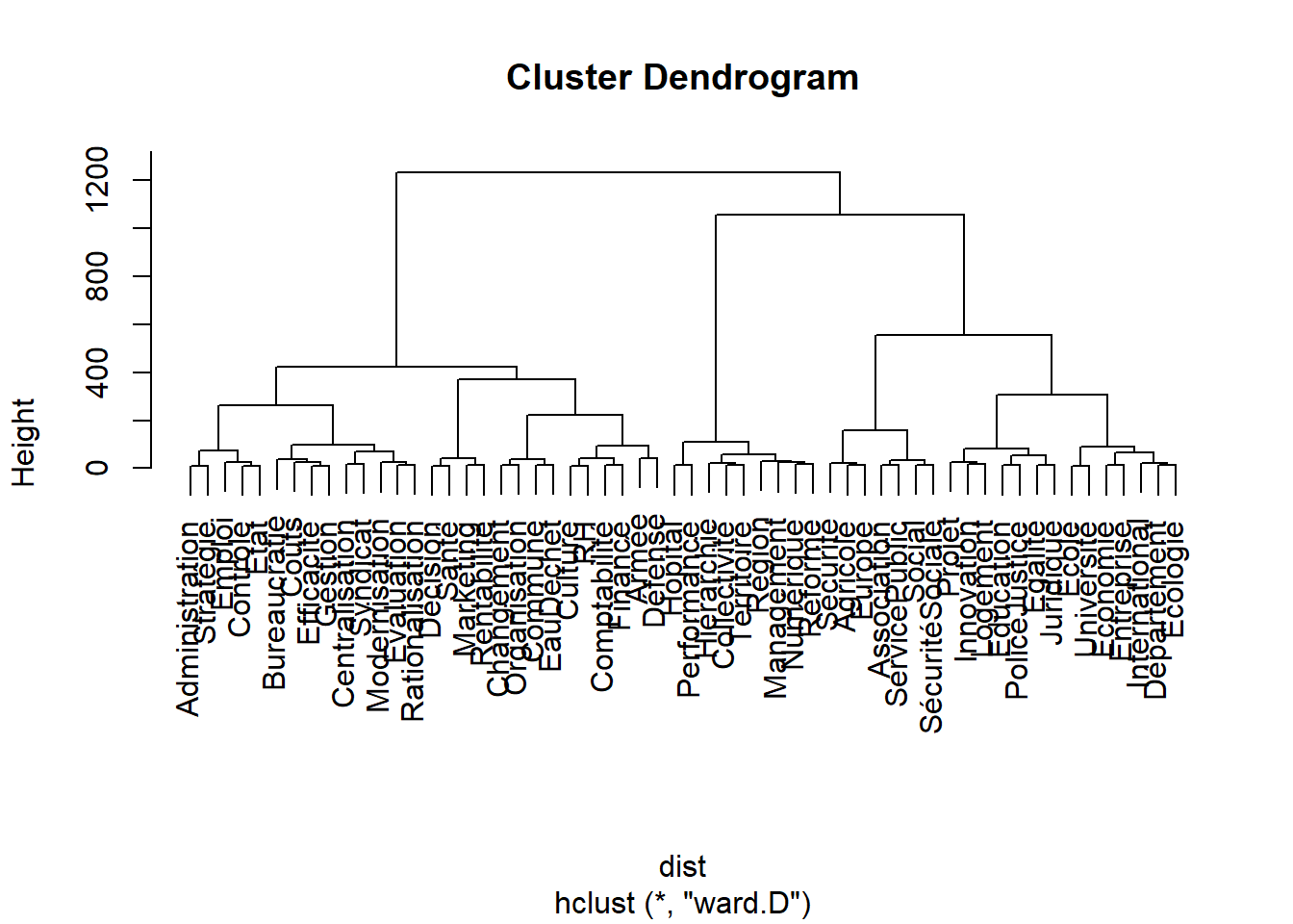
dist<-dist(TSNE[,1:3])


cluster  <- hclust(dist, "ward.D", ) # "wrong"
plot(cluster)

Code
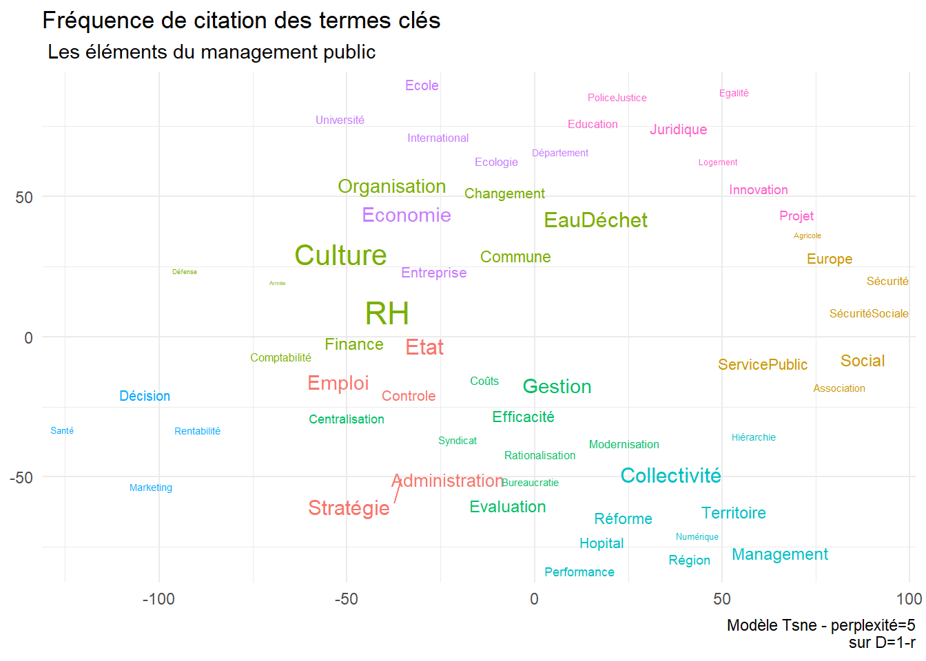
memb <- cutree(cluster, k = 8)
TSNE<-cbind(TSNE,memb)
TSNE$V1<-as.numeric(TSNE$V1)
TSNE$V2<-as.numeric(TSNE$V2)
ggplot(TSNE,aes(x=V1, y=V2,label=keyword))+
  geom_text_repel(aes(label=keyword,color=as.factor(memb),size=Densité), max.overlaps=Inf)+
  theme(legend.position="none")+
  labs(title="Fréquence de citation des termes clés",
       subtitle=" Les éléments du management public",
       x=NULL, y=NULL,
       caption = "Modèle Tsne - perplexité=5\nsur D=1-r")

Code
ggsave("./images/keyword50.jpeg", width = 27, height = 18, units = "cm")

typologie des papiers